Tecniche di stima - Guida rapida

Estimation è il processo di ricerca di una stima, o approssimazione, che è un valore che può essere utilizzato per qualche scopo anche se i dati di input possono essere incompleti, incerti o instabili.

La stima determina quanti soldi, impegno, risorse e tempo occorreranno per costruire un sistema o prodotto specifico. La stima si basa su -

• Dati passati / Esperienza passata
• Documenti / conoscenze disponibili
• Assumptions
• Rischi identificati

I quattro passaggi fondamentali nella stima del progetto software sono:

• Stimare le dimensioni del prodotto di sviluppo.
• Stimare lo sforzo in mesi-persona o ore-persona.
• Stima la pianificazione in mesi di calendario.
• Stimare il costo del progetto nella valuta concordata.

Osservazioni sulla stima

• La stima non deve essere un'attività una tantum in un progetto. Può avvenire durante:

  • Acquisizione di un progetto.
  • Pianificazione del progetto.
  • Esecuzione del progetto in caso di necessità.

• L'ambito del progetto deve essere compreso prima dell'inizio del processo di stima. Sarà utile avere i dati storici del progetto.

• Le metriche di progetto possono fornire una prospettiva storica e un input prezioso per la generazione di stime quantitative.

• La pianificazione richiede ai responsabili tecnici e al team del software di prendere un impegno iniziale in quanto porta alla responsabilità e alla responsabilità.

• L'esperienza passata può essere di grande aiuto.

• Utilizzare almeno due tecniche di stima per arrivare alle stime e riconciliare i valori risultanti. Fare riferimento a Tecniche di decomposizione nella sezione successiva per informazioni sulla riconciliazione delle stime.

• I piani dovrebbero essere iterativi e consentire aggiustamenti con il passare del tempo e più dettagli sono noti.

Approccio generale alla stima del progetto

L'approccio alla stima del progetto ampiamente utilizzato è Decomposition Technique. Le tecniche di decomposizione adottano un approccio divide et impera. La stima delle dimensioni, dell'impegno e dei costi viene eseguita in modo graduale suddividendo un progetto in funzioni principali o attività di ingegneria del software correlate.

Step 1 - Comprendere l'ambito del software da creare.

Step 2 - Genera una stima delle dimensioni del software.

• Inizia con la dichiarazione di ambito.

• Scomponi il software in funzioni che possono essere valutate individualmente.

• Calcola la dimensione di ciascuna funzione.

• Ricava stime di impegno e costi applicando i valori delle dimensioni alle metriche di produttività di base.

• Combina le stime delle funzioni per produrre una stima complessiva per l'intero progetto.

Step 3- Genera una stima dello sforzo e del costo. È possibile arrivare alle stime degli sforzi e dei costi suddividendo un progetto in attività di ingegneria del software correlate.

• Identificare la sequenza di attività che devono essere eseguite per completare il progetto.

• Dividi le attività in compiti che possono essere misurati.

• Stimare lo sforzo (in ore / giorni di persona) richiesto per completare ogni attività.

• Combina le stime dello sforzo delle attività dell'attività per produrre una stima per l'attività.

• Ottieni unità di costo (cioè costo / impegno unitario) per ciascuna attività dal database.

• Calcola lo sforzo totale e il costo per ciascuna attività.

• Combina le stime degli sforzi e dei costi per ciascuna attività per produrre uno sforzo complessivo e una stima dei costi per l'intero progetto.

Step 4- Riconcilia le stime: confronta i valori risultanti dal passaggio 3 con quelli ottenuti dal passaggio 2. Se entrambe le serie di stime concordano, i numeri sono altamente affidabili. Altrimenti, se si verificano stime ampiamente divergenti, condurre ulteriori indagini per verificare se:

• Lo scopo del progetto non è stato adeguatamente compreso o è stato interpretato male.

• La ripartizione delle funzioni e / o delle attività non è accurata.

• I dati storici utilizzati per le tecniche di stima non sono appropriati per l'applicazione, sono obsoleti o sono stati applicati in modo errato.

Step 5 - Determinare la causa della divergenza e quindi riconciliare le stime.

Precisione della stima

La precisione è un'indicazione di quanto qualcosa sia vicino alla realtà. Ogni volta che generi una stima, tutti vogliono sapere quanto i numeri sono vicini alla realtà. Vorrai che ogni stima sia il più accurata possibile, dati i dati che hai al momento della generazione. E ovviamente non vuoi presentare una stima in un modo che ispira un falso senso di fiducia nei numeri.

I fattori importanti che influenzano l'accuratezza delle stime sono:

• La precisione di tutti i dati di input della stima.

• La precisione di qualsiasi calcolo di stima.

• Quanto i dati storici oi dati di settore utilizzati per calibrare il modello corrispondono al progetto che stai stimando.

• La prevedibilità del processo di sviluppo del software della tua organizzazione.

• La stabilità sia dei requisiti del prodotto che dell'ambiente che supporta lo sforzo di ingegneria del software.

• Indipendentemente dal fatto che il progetto reale sia stato attentamente pianificato, monitorato e controllato e non si sono verificate grandi sorprese che hanno causato ritardi imprevisti.

Di seguito sono riportate alcune linee guida per ottenere stime affidabili:

• Stime di base su progetti simili che sono già stati completati.
• Utilizzare tecniche di scomposizione relativamente semplici per generare stime dei costi e degli sforzi del progetto.
• Utilizzare uno o più modelli di stima empirici per la stima dei costi e degli sforzi del software.

Fare riferimento alla sezione sulle Linee guida per la stima in questo capitolo.

Per garantire l'accuratezza, si consiglia sempre di stimare utilizzando almeno due tecniche e confrontare i risultati.

Problemi di stima

Spesso, i project manager ricorrono alla stima dei programmi saltando per stimare le dimensioni. Ciò può essere dovuto alle tempistiche stabilite dal top management o dal team di marketing. Tuttavia, qualunque sia la ragione, se ciò viene fatto, in una fase successiva sarebbe difficile stimare i programmi per accogliere i cambiamenti dell'ambito.

Durante la stima, possono essere fatte alcune ipotesi. È importante notare tutte queste ipotesi nel foglio di stima, poiché alcune ancora non documentano le ipotesi nei fogli di stima.

Anche buone stime hanno presupposti, rischi e incertezza intrinseci, eppure sono spesso trattate come se fossero accurate.

Il modo migliore per esprimere le stime è come una serie di possibili risultati dicendo, ad esempio, che il progetto richiederà dai 5 ai 7 mesi invece di affermare che sarà completo in una data particolare o sarà completato in un numero fisso. di mesi. Attenzione a impegnarsi in un intervallo troppo ristretto in quanto equivale a impegnarsi in una data definita.

• Potresti anche includere l'incertezza come valore di probabilità associato. Ad esempio, esiste una probabilità del 90% che il progetto venga completato entro una data definita.

• Le organizzazioni non raccolgono dati di progetto accurati. Poiché l'accuratezza delle stime dipende dai dati storici, sarebbe un problema.

• Per qualsiasi progetto, esiste una pianificazione più breve possibile che ti consentirà di includere le funzionalità richieste e produrre risultati di qualità. Se esiste un vincolo di pianificazione da parte della direzione e / o del cliente, è possibile negoziare l'ambito e la funzionalità da fornire.

• Concordare con il cliente sulla gestione dei creep dell'ambito per evitare superamenti del programma.

• L'incapacità di accogliere gli imprevisti nella stima finale causa problemi. Ad esempio, riunioni, eventi organizzativi.

• L'utilizzo delle risorse dovrebbe essere considerato inferiore all'80%. Questo perché le risorse sarebbero produttive solo per l'80% del loro tempo. Se si assegnano risorse con un utilizzo superiore all'80%, è inevitabile che si verifichino degli slittamenti.

Linee guida per la stima

Si dovrebbero tenere a mente le seguenti linee guida durante la stima di un progetto:

• Durante la stima, chiedi le esperienze di altre persone. Inoltre, metti le tue esperienze al lavoro.

• Supponiamo che le risorse saranno produttive solo per l'80% del loro tempo. Pertanto, durante la stima, considerare l'utilizzo delle risorse inferiore all'80%.

• Le risorse che lavorano su più progetti richiedono più tempo per completare le attività a causa del tempo perso per passare da uno all'altro.

• Includere il tempo di gestione in ogni stima.

• Costruisci sempre le contingenze per la risoluzione di problemi, riunioni e altri eventi imprevisti.

• Concedi abbastanza tempo per fare una stima adeguata del progetto. Le stime affrettate sono stime imprecise e ad alto rischio. Per i grandi progetti di sviluppo, la fase di stima dovrebbe davvero essere considerata come un mini progetto.

• Ove possibile, utilizza dati documentati da progetti precedenti simili della tua organizzazione. Risulterà nella stima più accurata. Se la tua organizzazione non ha conservato i dati storici, ora è un buon momento per iniziare a raccoglierli.

• Utilizza stime basate sugli sviluppatori, poiché le stime preparate da persone diverse da quelle che faranno il lavoro saranno meno accurate.

• Utilizzare diverse persone per stimare e utilizzare diverse tecniche di stima.

• Riconcilia le stime. Osservare la convergenza o la diffusione tra le stime. Convergenza significa che hai una buona stima. La tecnica Wideband-Delphi può essere utilizzata per raccogliere e discutere le stime utilizzando un gruppo di persone, con l'intenzione di produrre una stima accurata e imparziale.

• Rivalutare il progetto più volte durante il suo ciclo di vita.

UN Function Point(FP) è un'unità di misura per esprimere la quantità di funzionalità aziendale che un sistema informativo (come prodotto) fornisce a un utente. I FP misurano le dimensioni del software. Sono ampiamente accettati come standard del settore per il dimensionamento funzionale.

Per il dimensionamento del software basato su FP, sono emersi numerosi standard riconosciuti e / o specifiche pubbliche. A partire dal 2013, questi sono:

Standard ISO

• COSMIC- ISO / IEC 19761: 2011 Ingegneria del software. Un metodo di misurazione della taglia funzionale.

• FiSMA - ISO / IEC 29881: 2008 Tecnologia dell'informazione - Software e ingegneria dei sistemi - Metodo di misurazione della dimensione funzionale FiSMA 1.1.

• IFPUG - ISO / IEC 20926: 2009 Software e ingegneria dei sistemi - Misurazione del software - Metodo di misurazione della dimensione funzionale IFPUG.

• Mark-II - ISO / IEC 20968: 2002 Ingegneria del software - Analisi dei punti funzionali Ml II - Manuale delle pratiche di conteggio.

• NESMA - ISO / IEC 24570: 2005 Ingegneria del software - Metodo di misurazione della dimensione della funzione NESMA versione 2.1 - Definizioni e linee guida per il conteggio per l'applicazione dell'analisi dei punti di funzione.

Specifica del gruppo di gestione degli oggetti per il punto funzione automatizzato

Object Management Group (OMG), un consorzio di standard del settore informatico a partecipazione aperta e senza scopo di lucro, ha adottato la specifica AFP (Automated Function Point) guidata dal Consortium for IT Software Quality. Fornisce uno standard per l'automazione del conteggio FP secondo le linee guida dell'International Function Point User Group (IFPUG).

Function Point Analysis (FPA) techniquequantifica le funzioni contenute nel software in termini significativi per gli utenti del software. I FP considerano il numero di funzioni sviluppate in base alla specifica dei requisiti.

Function Points (FP) Countingè regolato da un insieme standard di regole, processi e linee guida come definito dall'International Function Point Users Group (IFPUG). Questi sono pubblicati in Counting Practices Manual (CPM).

Storia dell'analisi dei punti di funzione

Il concetto di Function Points è stato introdotto da Alan Albrecht di IBM nel 1979. Nel 1984, Albrecht ha perfezionato il metodo. Le prime Linee guida per i punti di funzione furono pubblicate nel 1984. L'International Function Point Users Group (IFPUG) è un'organizzazione mondiale di utenti del software metrico Function Point Analysis con sede negli Stati Uniti. IlInternational Function Point Users Group (IFPUG)è un'organizzazione senza scopo di lucro, governata da membri fondata nel 1986. IFPUG possiede Function Point Analysis (FPA) come definito nello standard ISO 20296: 2009 che specifica le definizioni, le regole e le fasi per l'applicazione del metodo di misurazione della dimensione funzionale (FSM) dell'IFPUG. L'IFPUG mantiene il manuale CPM (Function Point Counting Practices). CPM 2.0 è stato rilasciato nel 1987 e da allora ci sono state diverse iterazioni. La versione 4.3 di CPM risale al 2010.

La versione 4.3.1 di CPM con le revisioni editoriali ISO incorporate risale al 2010. Lo standard ISO (IFPUG FSM) - Functional Size Measurement che fa parte di CPM 4.3.1 è una tecnica per misurare il software in termini di funzionalità che fornisce. Il CPM è uno standard approvato a livello internazionale secondo ISO / IEC 14143-1 Information Technology - Software Measurement.

Processo elementare (EP)

Il processo elementare è la più piccola unità di requisito funzionale dell'utente che:

• È significativo per l'utente.
• Costituisce una transazione completa.
• È autonomo e lascia l'attività dell'applicazione che viene conteggiata in uno stato coerente.

Funzioni

Esistono due tipi di funzioni:

• Funzioni dati
• Funzioni di transazione

Funzioni dati

Esistono due tipi di funzioni dati:

• File logici interni
• File di interfaccia esterna

Le funzioni dati sono costituite da risorse interne ed esterne che agiscono sul sistema.

Internal Logical Files

Il file logico interno (ILF) è un gruppo identificabile dall'utente di dati o informazioni di controllo correlati logicamente che risiedono interamente all'interno del limite dell'applicazione. L'intento principale di un ILF è conservare i dati mantenuti attraverso uno o più processi elementari dell'applicazione da contare. Un ILF ha il significato intrinseco di essere mantenuto internamente, ha una struttura logica ed è memorizzato in un file. (Fare riferimento alla Figura 1)

External Interface Files

External Interface File (EIF) è un gruppo identificabile dall'utente di dati logicamente correlati o informazioni di controllo che viene utilizzato dall'applicazione solo a scopo di riferimento. I dati risiedono interamente al di fuori del limite dell'applicazione e vengono mantenuti in un ILF da un'altra applicazione. Un FEI ha il significato intrinseco di essere mantenuto esternamente, è necessario sviluppare un'interfaccia per ottenere i dati dal file. (Fare riferimento alla Figura 1)

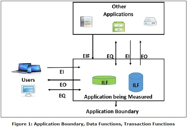
Funzioni di transazione

Esistono tre tipi di funzioni di transazione.

• Ingressi esterni
• Uscite esterne
• Richieste esterne

Le funzioni di transazione sono costituite dai processi che vengono scambiati tra l'utente, le applicazioni esterne e l'applicazione misurata.

External Inputs

L'input esterno (EI) è una funzione di transazione in cui i dati entrano "nell'applicazione" dall'esterno del confine verso l'interno. Questi dati provengono dall'esterno dell'applicazione.

• I dati possono provenire da una schermata di immissione dati o da un'altra applicazione.
• Un EI è il modo in cui un'applicazione ottiene le informazioni.
• I dati possono essere informazioni di controllo o informazioni aziendali.
• I dati possono essere utilizzati per mantenere uno o più file logici interni.
• Se i dati sono informazioni di controllo, non è necessario aggiornare un file logico interno. (Fare riferimento alla Figura 1)

External Outputs

L'output esterno (EO) è una funzione di transazione in cui i dati escono dal sistema. Inoltre, un EO può aggiornare un ILF. I dati creano report o file di output inviati ad altre applicazioni. (Fare riferimento alla Figura 1)

External Inquiries

External Inquiry (EQ) è una funzione di transazione con componenti sia di input che di output che determinano il recupero dei dati. (Fare riferimento alla Figura 1)

Definizione di RET, DET, FTR

Tipo di elemento record

Un Record Element Type (RET) è il più grande sottogruppo di elementi identificabili dall'utente all'interno di un ILF o di un EIF. È meglio esaminare i raggruppamenti logici di dati per identificarli.

Tipo di elemento dati

Data Element Type (DET) è il sottogruppo di dati all'interno di un FTR. Sono univoci e identificabili dall'utente.

Tipo di file referenziato

File Type Referenced (FTR) è il più grande sottogruppo identificabile dall'utente all'interno di EI, EO o EQ a cui si fa riferimento.

Le funzioni di transazione EI, EO, EQ vengono misurate contando FTR e DET che contengono seguendo le regole di conteggio. Allo stesso modo, le funzioni dati ILF e EIF vengono misurate contando DET e RET che contengono seguendo le regole di conteggio. Le misure delle funzioni di transazione e delle funzioni dati vengono utilizzate nel conteggio FP che risulta nella dimensione funzionale o nei punti funzione.

Il processo di conteggio FP prevede i seguenti passaggi:

• Step 1 - Determina il tipo di conteggio.

• Step 2 - Determina il limite del conteggio.

• Step 3 - Identificare ogni processo elementare (EP) richiesto dall'utente.

• Step 4 - Determina gli EP unici.

• Step 5 - Misura le funzioni dei dati.

• Step 6 - Misura le funzioni transazionali.

• Step 7 - Calcola la dimensione funzionale (conteggio dei punti funzione non aggiustato).

• Step 8 - Determinare il fattore di regolazione del valore (VAF).

• Step 9 - Calcola il conteggio dei punti funzione regolato.

Note- Le caratteristiche generali del sistema (GSC) sono rese opzionali in CPM 4.3.1 e spostate nell'appendice. Quindi, il passaggio 8 e il passaggio 9 possono essere saltati.

Passaggio 1: determinare il tipo di conteggio

Esistono tre tipi di conteggio dei punti funzione:

• Conteggio punti funzione di sviluppo
• Conteggio punti funzione applicazione
• Conteggio punti funzione di miglioramento

Conteggio punti funzione di sviluppo

I punti funzione possono essere conteggiati in tutte le fasi di un progetto di sviluppo, dal requisito alla fase di implementazione. Questo tipo di conteggio è associato al nuovo lavoro di sviluppo e può includere i prototipi, che potrebbero essere stati richiesti come soluzione temporanea, che supporta lo sforzo di conversione. Questo tipo di conteggio è chiamato conteggio di punti funzione di base.

Conteggio punti funzione applicazione

I conteggi delle applicazioni vengono calcolati come i punti funzione forniti ed escludono qualsiasi sforzo di conversione (prototipi o soluzioni temporanee) e funzionalità esistenti che potrebbero essere esistite.

Conteggio punti funzione di miglioramento

Quando vengono apportate modifiche al software dopo la produzione, vengono considerate miglioramenti. Per ridimensionare tali progetti di miglioramento, il conteggio dei punti funzione viene aggiunto, modificato o eliminato nell'applicazione.

Passaggio 2: determinare il limite del conteggio

Il confine indica il confine tra l'applicazione misurata e le applicazioni esterne o il dominio dell'utente. (Fare riferimento alla Figura 1)

Per determinare il confine, capire:

• Lo scopo del conteggio dei punti funzione
• Ambito dell'applicazione da misurare
• Come e quali applicazioni conservano quali dati
• Le aree di business che supportano le applicazioni

Passaggio 3: identificare ogni processo elementare richiesto dall'utente

Comporre e / o scomporre i requisiti utente funzionali nella più piccola unità di attività, che soddisfa tutti i seguenti criteri:

• È significativo per l'utente.
• Costituisce una transazione completa.
• È autonomo.
• Lascia l'attività dell'applicazione che viene conteggiata in uno stato coerente.

Ad esempio, il Requisito utente funzionale - "Mantieni informazioni sui dipendenti" può essere scomposto in attività più piccole come aggiungere dipendente, cambiare dipendente, eliminare dipendente e informarsi sul dipendente.

Ogni unità di attività così identificata è un Processo Elementare (EP).

Passaggio 4: determinare i processi elementari unici

Confrontando due EP già identificati, contarli come un EP (stesso EP) se:

• Richiede lo stesso set di DET.
• Richiedi lo stesso set di FTR.
• Richiede lo stesso set di logica di elaborazione per completare il PE.

Non dividere un EP con più forme di logica di elaborazione in più Eps.

Ad esempio, se hai identificato "Aggiungi dipendente" come EP, non dovrebbe essere diviso in due EP per tenere conto del fatto che un dipendente può o meno avere dipendenti. Il PE è ancora "Aggiungi dipendente" e vi sono variazioni nella logica di elaborazione e nei DET per tenere conto dei dipendenti.

Passaggio 5: misurare le funzioni dei dati

Classificare ogni funzione dati come ILF o EIF.

Una funzione dati è classificata come:

• File logico interno (ILF), se mantenuto dall'applicazione misurata.

• File di interfaccia esterna (EIF) se è referenziato, ma non mantenuto dall'applicazione misurata.

Gli ILF e gli EIF possono contenere dati aziendali, dati di controllo e dati basati su regole. Ad esempio, la commutazione del telefono è composta da tutti e tre i tipi: dati aziendali, dati delle regole e dati di controllo. I dati aziendali sono la vera chiamata. I dati delle regole sono il modo in cui la chiamata deve essere instradata attraverso la rete, mentre i dati di controllo sono il modo in cui gli interruttori comunicano tra loro.

Considera la seguente documentazione per il conteggio di ILF e FEI:

• Obiettivi e vincoli per il sistema proposto.
• Documentazione relativa al sistema attuale, se tale sistema esiste.
• Documentazione degli obiettivi, dei problemi e dei bisogni percepiti dagli utenti.
• Modelli di dati.

Passaggio 5.1: contare i DET per ciascuna funzione dati

Applicare le seguenti regole per contare i DET per ILF / EIF:

• Contare un DET per ogni campo identificabile dall'utente univoco, non ripetuto mantenuto o recuperato dall'ILF o EIF attraverso l'esecuzione di un EP.

• Contare solo i DET utilizzati dall'applicazione misurati quando due o più applicazioni mantengono e / o fanno riferimento alla stessa funzione dati.

• Contare un DET per ogni attributo richiesto dall'utente per stabilire una relazione con un altro ILF o EIF.

• Rivedere gli attributi correlati per determinare se sono raggruppati e conteggiati come un singolo DET o se sono conteggiati come più DET. Il raggruppamento dipenderà da come gli EP utilizzano gli attributi all'interno dell'applicazione.

Passaggio 5.2: contare i RET per ciascuna funzione dati

Applicare le seguenti regole per contare i RET per ILF / EIF:

• Contare un RET per ogni funzione dati.
• Contare un RET aggiuntivo per ciascuno dei seguenti sottogruppi logici aggiuntivi di DET.
  • Entità associativa con attributi non chiave.
  • Sottotipo (diverso dal primo sottotipo).
  • Entità attributiva, in una relazione diversa da quella obbligatoria 1: 1.

Passaggio 5.3: determinare la complessità funzionale per ciascuna funzione dati

RETS	Tipi di elementi dati (DET)
	1-19	20-50	>50
1	L	L	UN
Da 2 a 5	L	UN	H
> 5	UN	H	H

Complessità funzionale: L = Basso; A = Media; H = Alto

Passaggio 5.4: misurare la dimensione funzionale per ciascuna funzione dati

Complessità funzionale	Conteggio FP per ILF	Conteggio FP per FEI
Basso	7	5
Media	10	7
Alto	15	10

Passaggio 6: misurare le funzioni transazionali

Per misurare le funzioni transazionali, i seguenti sono i passaggi necessari:

Passaggio 6.1: classificare ciascuna funzione transazionale

Le funzioni transazionali dovrebbero essere classificate come Input esterno, Output esterno o Indagine esterna.

Ingresso esterno

L'input esterno (EI) è un processo elementare che elabora i dati o controlla le informazioni che provengono dall'esterno del confine. Lo scopo principale di un'IE è quello di mantenere uno o più ILF e / o alterare il comportamento del sistema.

Devono essere applicate tutte le seguenti regole:

• I dati o le informazioni di controllo vengono ricevuti dall'esterno del limite dell'applicazione.

• Almeno un ILF viene mantenuto se i dati che entrano nel confine non sono informazioni di controllo che alterano il comportamento del sistema.

• Per il PE identificato, deve essere applicata una delle tre dichiarazioni:

  • La logica di elaborazione è unica rispetto alla logica di elaborazione eseguita da altri EI per l'applicazione.

  • La serie di elementi di dati identificati è diversa dalle serie identificate per altri EI nell'applicazione.

  • Gli ILF o EIF a cui si fa riferimento sono diversi dai file a cui fanno riferimento gli altri EI nella domanda.

Uscita esterna

L'output esterno (EO) è un processo elementare che invia dati o informazioni di controllo al di fuori dei confini dell'applicazione. EO include un'elaborazione aggiuntiva oltre a quella di un'indagine esterna.

Lo scopo principale di un EO è presentare le informazioni a un utente attraverso una logica di elaborazione diversa o in aggiunta al recupero di dati o informazioni di controllo.

La logica di elaborazione deve:

• Contenere almeno una formula matematica o un calcolo.
• Crea dati derivati.
• Mantieni uno o più ILF.
• Modifica il comportamento del sistema.

Devono essere applicate tutte le seguenti regole:

• Invia dati o informazioni di controllo esterne al limite dell'applicazione.
• Per il PE identificato, deve essere applicata una delle tre dichiarazioni:
  • La logica di elaborazione è unica rispetto alla logica di elaborazione eseguita da altri EO per l'applicazione.
  • L'insieme di elementi di dati identificato è diverso dagli altri EO nell'applicazione.
  • Gli ILF o EIF a cui si fa riferimento sono diversi dai file a cui fanno riferimento altri EO nell'applicazione.

Inoltre, deve essere applicata una delle seguenti regole:

• La logica di elaborazione contiene almeno una formula matematica o un calcolo.
• La logica di elaborazione mantiene almeno un ILF.
• La logica di elaborazione altera il comportamento del sistema.

Indagine esterna

L'indagine esterna (EQ) è un processo elementare che invia dati o informazioni di controllo al di fuori del confine. Lo scopo principale di un EQ è presentare le informazioni all'utente attraverso il recupero di dati o informazioni di controllo.

La logica di elaborazione non contiene formule matematiche o calcoli e non crea dati derivati. Nessun ILF viene mantenuto durante l'elaborazione, né il comportamento del sistema viene alterato.

Devono essere applicate tutte le seguenti regole:

• Invia dati o informazioni di controllo esterne al limite dell'applicazione.
• Per il PE identificato, deve essere applicata una delle tre dichiarazioni:
  • La logica di elaborazione è unica rispetto alla logica di elaborazione eseguita da altri EQ per l'applicazione.
  • L'insieme di elementi di dati identificati è diverso dagli altri EQ nell'applicazione.
  • Gli ILF o EIF a cui si fa riferimento sono diversi dai file a cui fanno riferimento altri EQ nell'applicazione.

Inoltre, devono essere applicate tutte le seguenti regole:

• La logica di elaborazione recupera i dati o le informazioni di controllo da un ILF o EIF.
• La logica di elaborazione non contiene formule matematiche o calcoli.
• La logica di elaborazione non altera il comportamento del sistema.
• La logica di elaborazione non mantiene un ILF.

Passaggio 6.2: contare i DET per ciascuna funzione transazionale

Applicare le seguenti regole per contare i DET per gli EI:

• Rivedi tutto ciò che attraversa (entra e / o esce) il confine.

• Contare un DET per ogni attributo identificabile e non ripetuto univoco dell'utente che attraversa (entra e / o esce) il confine durante l'elaborazione della funzione transazionale.

• Contare solo un DET per funzione transazionale per la capacità di inviare un messaggio di risposta dell'applicazione, anche se sono presenti più messaggi.

• Contare solo un DET per funzione transazionale per la capacità di avviare azioni anche se ci sono più mezzi per farlo.

• Non contare i seguenti elementi come DET:

  • Attributi generati all'interno del confine da una funzione transazionale e salvati in un ILF senza uscire dal confine.

  • Valori letterali come titoli di report, identificatori di schermate o pannelli, intestazioni di colonne e titoli di attributi.

  • Timbri generati dall'applicazione come attributi di data e ora.

  • Variabili di paginazione, numeri di pagina e informazioni sul posizionamento, ad esempio, "Righe da 37 a 54 di 211".

  • Aiuti alla navigazione come la possibilità di navigare all'interno di un elenco utilizzando "precedente", "successivo", "primo", "ultimo" e i loro equivalenti grafici.

Applicare le seguenti regole per contare i DET per EO / EQ:

• Rivedi tutto ciò che attraversa (entra e / o esce) il confine.

• Contare un DET per ogni attributo identificabile e non ripetuto univoco dell'utente che attraversa (entra e / o esce) il confine durante l'elaborazione della funzione transazionale.

• Contare solo un DET per funzione transazionale per la capacità di inviare un messaggio di risposta dell'applicazione, anche se sono presenti più messaggi.

• Contare solo un DET per funzione transazionale per la capacità di avviare azioni anche se ci sono più mezzi per farlo.

• Non contare i seguenti elementi come DET:

  • Attributi generati all'interno del confine senza attraversare il confine.

  • Valori letterali come titoli di report, identificatori di schermate o pannelli, intestazioni di colonne e titoli di attributi.

  • Timbri generati dall'applicazione come attributi di data e ora.

  • Variabili di paginazione, numeri di pagina e informazioni sul posizionamento, ad esempio, "Righe da 37 a 54 di 211".

  • Aiuti alla navigazione come la possibilità di navigare all'interno di un elenco utilizzando "precedente", "successivo", "primo", "ultimo" e i loro equivalenti grafici.

Passaggio 6.3: contare gli FTR per ciascuna funzione transazionale

Applica le seguenti regole per contare gli FTR per gli EI:

• Contare un FTR per ogni ILF mantenuto.
• Contare un FTR per ogni lettura ILF o EIF durante l'elaborazione dell'EI.
• Contare solo un FTR per ogni ILF che viene mantenuto e letto.

Applica la seguente regola per contare gli FTR per EO / EQ:

• Contare un FTR per ogni lettura ILF o EIF durante l'elaborazione di EP.

Inoltre, applica le seguenti regole per contare gli FTR per gli EO:

• Contare un FTR per ogni ILF mantenuto durante l'elaborazione di EP.
• Contare solo un FTR per ogni ILF che viene mantenuto e letto da EP.

Passaggio 6.4: determinare la complessità funzionale per ciascuna funzione transazionale

FTR	Tipi di elementi dati (DET)
	1-4	5-15	>=16
0-1	L	L	UN
2	L	UN	H
> = 3	UN	H	H

Complessità funzionale: L = Basso; A = Media; H = Alto

Determina la complessità funzionale per ogni EO / EQ, con l'eccezione che l'EQ deve avere un minimo di 1 FTR -

L'EQ deve avere un minimo di 1 FTR FTR	Tipi di elementi dati (DET)
	1-4	5-15	> = 16
0-1	L	L	UN
2	L	UN	H
> = 3	UN	H	H

Complessità funzionale: L = Basso; A = Media; H = Alto

Passaggio 6.5: misurare la dimensione funzionale per ciascuna funzione transazionale

Misurare la dimensione funzionale per ogni EI dalla sua complessità funzionale.

Complessità	Conteggio FP
Basso	3
Media	4
Alto	6

Misura la dimensione funzionale per ogni EO / EQ dalla sua complessità funzionale.

Complessità	Conteggio FP per EO	Conteggio FP per EQ
Basso	4	3
Media	5	4
Alto	6	6

Passaggio 7: calcolare la dimensione funzionale (conteggio punti funzione non regolato)

Per calcolare la dimensione funzionale, è necessario seguire i passaggi indicati di seguito:

Passaggio 7.1

Ricorda cosa hai trovato nel passaggio 1. Determina il tipo di conteggio.

Passaggio 7.2

Calcola la dimensione funzionale o il conteggio dei punti funzione in base al tipo.

• Per il conteggio dei punti della funzione di sviluppo, andare al passaggio 7.3.
• Per il conteggio dei punti funzione dell'applicazione, andare al passaggio 7.4.
• Per il conteggio dei punti della funzione di miglioramento, andare al passaggio 7.5.

Passaggio 7.3

Il conteggio dei punti della funzione di sviluppo consiste di due componenti di funzionalità:

• Funzionalità dell'applicazione inclusa nei requisiti utente per il progetto.

• Funzionalità di conversione inclusa nei requisiti utente per il progetto. La funzionalità di conversione consiste in funzioni fornite solo durante l'installazione per convertire i dati e / o fornire altri requisiti di conversione specificati dall'utente, come rapporti di conversione speciali. Ad esempio, un'applicazione esistente può essere sostituita con un nuovo sistema.

DFP = ADD + CFP

Dove,

DFP = Conteggio punti funzione di sviluppo

ADD = Dimensioni delle funzioni fornite all'utente dal progetto di sviluppo

CFP = Dimensioni della funzionalità di conversione

ADD = Conteggio FP (ILF) + Conteggio FP (EIF) + Conteggio FP (EIs) + Conteggio FP (EO) + Conteggio FP (EQ)

CFP = Conteggio FP (ILF) + Conteggio FP (EIF) + Conteggio FP (EIs) + Conteggio FP (EO) + Conteggio FP (EQ)

Passaggio 7.4

Calcola il conteggio dei punti della funzione dell'applicazione

AFP = ADD

Dove,

AFP = Conteggio punti funzione applicazione

ADD = Dimensione delle funzioni fornite all'utente dal progetto di sviluppo (esclusa la dimensione di qualsiasi funzionalità di conversione) o la funzionalità che esiste ogni volta che viene conteggiata l'applicazione.

ADD = Conteggio FP (ILF) + Conteggio FP (EIF) + Conteggio FP (EIs) + Conteggio FP (EO) + Conteggio FP (EQ)

Passaggio 7.5

La funzione di miglioramento Point Count considera i seguenti quattro componenti della funzionalità:

• Funzionalità che viene aggiunta all'applicazione.
• Funzionalità che viene modificata nell'applicazione.
• Funzionalità di conversione.
• Funzionalità che viene eliminata dall'applicazione.

EFP = ADD + CHGA + CFP + DEL

Dove,

EFP = Conteggio punti funzione di miglioramento

ADD = Dimensioni delle funzioni aggiunte dal progetto di miglioramento

CHGA = Dimensioni delle funzioni modificate dal progetto di miglioramento

CFP = Dimensioni della funzionalità di conversione

DEL = Dimensioni delle funzioni eliminate dal progetto di miglioramento

ADD = Conteggio FP (ILF) + Conteggio FP (EIF) + Conteggio FP (EIs) + Conteggio FP (EO) + Conteggio FP (EQ)

CHGA = Conteggio FP (ILF) + Conteggio FP (EIF) + Conteggio FP (EIs) + Conteggio FP (EO) + Conteggio FP (EQ)

CFP = Conteggio FP (ILF) + Conteggio FP (EIF) + Conteggio FP (EIs) + Conteggio FP (EO) + Conteggio FP (EQ)

DEL = Conteggio FP (ILF) + Conteggio FP (EIF) + CONTO FP (EIs) + Conteggio FP (EO) + Conteggio FP (EQ)

Passaggio 8: determinare il fattore di regolazione del valore

Le GSC sono rese facoltative in CPM 4.3.1 e spostate nell'appendice. Quindi, il passaggio 8 e il passaggio 9 possono essere saltati.

Il Value Adjustment Factor (VAF) si basa su 14 GSC che valutano la funzionalità generale dell'applicazione da conteggiare. Le GSC sono vincoli aziendali degli utenti indipendenti dalla tecnologia. Ogni caratteristica ha descrizioni associate per determinare il grado di influenza.

Caratteristica generale del sistema	Breve descrizione
Comunicazioni di dati	Quante strutture di comunicazione ci sono per facilitare il trasferimento o lo scambio di informazioni con l'applicazione o il sistema?
Elaborazione dati distribuita	Come vengono gestiti i dati distribuiti e le funzioni di elaborazione?
Prestazione	L'utente ha richiesto tempo di risposta o velocità effettiva?
Configurazione molto usata	Quanto è utilizzata l'attuale piattaforma hardware su cui verrà eseguita l'applicazione?
Tasso di transazione	Con quale frequenza vengono eseguite le transazioni giornaliere, settimanali, mensili, ecc.?
Inserimento dati in linea	Quale percentuale delle informazioni viene inserita online?
Efficienza dell'utente finale	L'applicazione è stata progettata per l'efficienza dell'utente finale?
Aggiornamento in linea	Quanti ILF vengono aggiornati tramite transazione online?
Elaborazione complessa	L'applicazione dispone di un'ampia elaborazione logica o matematica?
Riusabilità	L'applicazione è stata sviluppata per soddisfare le esigenze di uno o più utenti?
Facilità di installazione	Quanto sono difficili la conversione e l'installazione?
Facilità operativa	Quanto sono efficaci e / o automatizzate le procedure di avvio, backup e ripristino?
Più siti	L'applicazione è stata progettata, sviluppata e supportata specificamente per essere installata in più siti per più organizzazioni?
Facilitare il cambiamento	L'applicazione è stata progettata, sviluppata e supportata specificamente per facilitare il cambiamento?

La gamma del grado di influenza è su una scala da zero a cinque, da nessuna influenza a forte influenza.

Valutazione	Grado di influenza
0	Non presente o nessuna influenza
1	Influenza accidentale
2	Influenza moderata
3	Influenza media
4	Influenza significativa
5	Forte influenza ovunque

Determina il grado di influenza per ciascuna delle 14 GSC.

La somma dei valori delle 14 GSC così ottenute è denominata Total Degree of Influence (TDI).

TDI = ∑¹⁴ Degrees of Influence

Quindi, calcola il fattore di regolazione del valore (VAF) come

VAF = (TDI × 0.01) + 0.65

Ogni GSC può variare da 0 a 5, TDI può variare da (0 × 14) a (5 × 14), cioè da 0 (quando tutte le GSC sono basse) a 70 (quando tutte le GSC sono alte) cioè 0 ≤ TDI ≤ 70. Quindi, VAF può variare nell'intervallo da 0,65 (quando tutte le GSC sono basse) a 1,35 (quando tutte le GSC sono alte), ovvero 0,65 ≤ VAF ≤ 1,35.

Passaggio 9: calcolare il conteggio dei punti funzione regolati

Secondo l'approccio FPA che utilizza il VAF (versioni CPM precedenti alla V4.3.1), questo è determinato da,

Adjusted FP Count = Unadjusted FP Count × VAF

Dove, il conteggio FP non corretto è la dimensione funzionale calcolata nel passaggio 7.

Poiché il VAF può variare da 0,65 a 1,35, il VAF esercita un'influenza del ± 35% sul conteggio FP finale regolato.

Vantaggi dei punti funzione

I punti funzione sono utili -

• Misurando la dimensione della soluzione invece della dimensione del problema.

• Poiché i requisiti sono l'unica cosa necessaria per il conteggio dei punti funzione.

• Poiché è indipendente dalla tecnologia.

• Poiché è indipendente dai linguaggi di programmazione.

• Nella stima dei progetti di test.

• Nella stima dei costi, della pianificazione e dell'impegno complessivi del progetto.

• Nelle trattative contrattuali in quanto fornisce un metodo di comunicazione più facile con i gruppi aziendali.

• Poiché quantifica e assegna un valore agli usi, alle interfacce e agli scopi effettivi delle funzioni nel software.

• Nella creazione di rapporti con altre metriche come ore, costo, organico, durata e altre metriche dell'applicazione.

Repository FP

International Software Benchmarking Standards Group (ISBSG) cresce e mantiene due archivi per i dati IT.

• Progetti di sviluppo e valorizzazione
• Applicazioni di manutenzione e supporto

Ci sono più di 6.000 progetti nel repository dei progetti di sviluppo e miglioramento.

I dati vengono forniti in formato Microsoft Excel, rendendo più facile per ulteriori analisi che si desidera eseguire con esso, o è anche possibile utilizzare i dati per qualche altro scopo.

La licenza del repository ISBSG può essere acquistata da: http://www.isbsg.com/

ISBSG offre uno sconto del 10% ai membri IFPUG per gli acquisti online quando viene utilizzato il codice sconto "IFPUGMembers".

Gli aggiornamenti del rilascio dei dati del progetto software ISBSG sono disponibili all'indirizzo: http://www.ifpug.org/isbsg/

COSMIC e IFPUG hanno collaborato alla produzione di un glossario di termini per requisiti software e non funzionali. Può essere scaricato da - cosmic-sizing.org

UN Use-Case è una serie di interazioni correlate tra un utente e un sistema che consente all'utente di raggiungere un obiettivo.

I casi d'uso sono un modo per acquisire i requisiti funzionali di un sistema. L'utente del sistema viene definito "attore". I casi d'uso sono fondamentalmente in forma di testo.

Punti del caso d'uso - Definizione

Use-Case Points (UCP)è una tecnica di stima del software utilizzata per misurare le dimensioni del software con casi d'uso. Il concetto di UCP è simile ai FP.

Il numero di UCP in un progetto si basa su quanto segue:

• Il numero e la complessità dei casi d'uso nel sistema.
• Il numero e la complessità degli attori del sistema.

  • Vari requisiti non funzionali (come portabilità, prestazioni, manutenibilità) che non sono scritti come casi d'uso.

  • L'ambiente in cui verrà sviluppato il progetto (come la lingua, la motivazione del team, ecc.)

La stima con gli UCP richiede che tutti i casi d'uso siano scritti con un obiettivo e approssimativamente allo stesso livello, fornendo la stessa quantità di dettagli. Quindi, prima della stima, il team di progetto dovrebbe assicurarsi di aver scritto i propri casi d'uso con obiettivi definiti ea livello dettagliato. Il caso d'uso viene normalmente completato in una singola sessione e una volta raggiunto l'obiettivo, l'utente può passare a qualche altra attività.

Storia dei casi d'uso

Il metodo di stima Use-Case Point è stato introdotto da Gustav Karner nel 1993. Il lavoro è stato successivamente concesso in licenza da Rational Software che si è fusa con IBM.

Processo di conteggio dei punti dei casi d'uso

Il processo di conteggio dei punti caso d'uso prevede i seguenti passaggi:

• Calcola gli UCP non aggiustati
• Adatta alla complessità tecnica
• Adeguare la complessità ambientale
• Calcola gli UCP aggiustati

Passaggio 1: calcolare i punti caso d'uso non regolati.

Calcola prima i punti caso d'uso non aggiustati, procedendo come segue:

• Determina il peso del caso d'uso non adattato
• Determina il peso dell'attore non aggiustato
• Calcola punti caso d'uso non regolati

Step 1.1 - Determina il peso del caso d'uso non adattato.

Step 1.1.1 - Trova il numero di transazioni in ogni caso d'uso.

Se i casi d'uso sono scritti con livelli di obiettivo utente, una transazione equivale a un passaggio nel caso d'uso. Trova il numero di transazioni contando i passaggi nel caso d'uso.

Step 1.1.2- Classificare ogni caso d'uso come semplice, medio o complesso in base al numero di transazioni nel caso d'uso. Inoltre, assegnare il peso del caso d'uso come mostrato nella tabella seguente:

Complessità dei casi d'uso	Numero di transazioni	Peso caso d'uso
Semplice	≤3	5
Media	Da 4 a 7	10
Complesso	> 7	15

Step 1.1.3- Ripeti per ogni caso d'uso e ottieni tutti i pesi dei casi d'uso. Il peso del caso d'uso non aggiustato (UUCW) è la somma di tutti i pesi del caso d'uso.

Step 1.1.4 - Trova il peso del caso d'uso non regolato (UUCW) utilizzando la seguente tabella -

Complessità dei casi d'uso	Peso caso d'uso	Numero di casi d'uso	Prodotto
Semplice	5	NSUC	5 × NSUC
Media	10	NAUC	10 × NAUC
Complesso	15	NCUC	15 × NCUC
Unadjusted Use-Case Weight (UUCW)			5 × NSUC + 10 × NAUC + 15 × NCUC

Dove,

NSUC è il no. di casi d'uso semplici.

NAUC è il no. di casi d'uso medi.

NCUC è il no. di casi d'uso complessi.

Step 1.2 - Determina il peso dell'attore non aggiustato.

Un attore in un caso d'uso potrebbe essere una persona, un altro programma, ecc. Alcuni attori, come un sistema con API definite, hanno esigenze molto semplici e aumentano solo leggermente la complessità di un caso d'uso.

Alcuni attori, come un sistema che interagisce tramite un protocollo, hanno più esigenze e aumentano la complessità di un caso d'uso in una certa misura.

Altri attori, come un utente che interagisce tramite la GUI, hanno un impatto significativo sulla complessità di un caso d'uso. Sulla base di queste differenze, puoi classificare gli attori come semplici, medi e complessi.

Step 1.2.1 - Classificare gli attori come semplici, medi e complessi e assegnare i pesi degli attori come mostrato nella tabella seguente -

Complessità dell'attore	Esempio	Peso dell'attore
Semplice	Un sistema con API definite	1
Media	Un sistema che interagisce tramite un protocollo	2
Complesso	Un utente che interagisce tramite GUI	3

Step 1.2.2- Ripeti per ogni attore e ottieni tutti i pesi degli attori. Peso attore non regolato (UAW) è la somma di tutti i pesi attore.

Step 1.2.3 - Trova il peso dell'attore non regolato (UAW) utilizzando la seguente tabella -

Complessità dell'attore	Peso dell'attore	Numero di attori	Prodotto
Semplice	1	NSA	1 × NSA
Media	2	NAA	2 × NAA
Complesso	3	NCA	3 × NCA
Unadjusted Actor Weight (UAW)			1 × NSA + 2 × NAA + 3 × NCA

Dove,

NSA è il no. di Simple Actors.

NAA è il no. di attori medi.

NCA è il no. di attori complessi.

Step 1.3 - Calcola punti caso d'uso non regolati.

L'Unadjusted Use-Case Weight (UUCW) e il Unadjusted Actor Weight (UAW) insieme danno la dimensione non aggiustata del sistema, denominata Unadjusted Use-Case Points.

Unadjusted Use-Case Points (UUCP) = UUCW + UAW

I passaggi successivi consistono nell'adeguare i punti del caso d'uso non adattato (UUCP) per complessità tecnica e complessità ambientale.

Passaggio 2: regolare la complessità tecnica

Step 2.1 - Considera i 13 fattori che contribuiscono all'impatto della complessità tecnica di un progetto sui punti del caso d'uso e i loro pesi corrispondenti come indicato nella tabella seguente -

Fattore	Descrizione	Peso
T1	Sistema distribuito	2.0
T2	Tempo di risposta o obiettivi di rendimento del throughput	1.0
T3	Efficienza dell'utente finale	1.0
T4	Elaborazione interna complessa	1.0
T5	Il codice deve essere riutilizzabile	1.0
T6	Facile da installare	.5
T7	Facile da usare	.5
T8	Portatile	2.0
T9	Facile da cambiare	1.0
T10	Concorrente	1.0
T11	Include obiettivi di sicurezza speciali	1.0
T12	Fornisce accesso diretto a terzi	1.0
T13	Sono necessarie speciali strutture per la formazione degli utenti	1.0

Molti di questi fattori rappresentano i requisiti non funzionali del progetto.

Step 2.2 - Per ciascuno dei 13 fattori, valutare il progetto e valutare da 0 (irrilevante) a 5 (molto importante).

Step 2.3 - Calcola l'impatto del fattore dal peso dell'impatto del fattore e il valore nominale per il progetto come

Impact of the Factor = Impact Weight × Rated Value

Step (2.4)- Calcola la somma dell'impatto di tutti i fattori. Questo dà il fattore tecnico totale (TFactor) come indicato nella tabella seguente:

Fattore	Descrizione	Peso (W)	Valore nominale (da 0 a 5) (RV)	Impatto (I = W × RV)
T1	Sistema distribuito	2.0
T2	Tempo di risposta o obiettivi di rendimento del throughput	1.0
T3	Efficienza dell'utente finale	1.0
T4	Elaborazione interna complessa	1.0
T5	Il codice deve essere riutilizzabile	1.0
T6	Facile da installare	.5
T7	Facile da usare	.5
T8	Portatile	2.0
T9	Facile da cambiare	1.0
T10	Concorrente	1.0
T11	Include obiettivi di sicurezza speciali	1.0
T12	Fornisce accesso diretto a terzi	1.0
T13	Sono necessarie speciali strutture per la formazione degli utenti	1.0
Total Technical Factor (TFactor)

Step 2.5 - Calcola il fattore di complessità tecnica (TCF) come -

TCF = 0.6 + (0.01 × TFactor)

Passaggio 3: adeguare la complessità ambientale

Step 3.1 - Considerare gli 8 fattori ambientali che potrebbero influenzare l'esecuzione del progetto e i loro pesi corrispondenti come indicato nella tabella seguente -

Fattore	Descrizione	Peso
F1	Familiarità con il modello di progetto utilizzato	1.5
F2	Esperienza applicativa	.5
F3	Esperienza orientata agli oggetti	1.0
F4	Capacità di analista principale	.5
F5	Motivazione	1.0
F6	Stable requirements	2.0
F7	Part-time staff	-1.0
F8	Difficult programming language	-1.0

Step 3.2 − For each of the 8 Factors, assess the project and rate from 0 (irrelevant) to 5 (very important).

Step 3.3 − Calculate the Impact of the Factor from Impact Weight of the Factor and the Rated Value for the project as

Impact of the Factor = Impact Weight × Rated Value

Step 3.4 − Calculate the sum of Impact of all the Factors. This gives the Total Environment Factor (EFactor) as given in the following table −

Factor	Description	Weight (W)	Rated Value (0 to 5) (RV)	Impact (I = W × RV)
F1	Familiar with the project model that is used	1.5
F2	Application experience	.5
F3	Object-oriented experience	1.0
F4	Lead analyst capability	.5
F5	Motivation	1.0
F6	Stable requirements	2.0
F7	Part-time staff	-1.0
F8	Difficult programming language	-1.0
Total Environment Factor (EFactor)

Step 3.5 − Calculate the Environmental Factor (EF) as −

1.4 + (-0.03 × EFactor)

Step 4: Calculate Adjusted Use-Case Points (UCP)

Calculate Adjusted Use-Case Points (UCP) as −

UCP = UUCP × TCF × EF

Advantages and Disadvantages of Use-Case Points

Advantages of Use-Case Points

• UCPs are based on use cases and can be measured very early in the project life cycle.

• UCP (size estimate) will be independent of the size, skill, and experience of the team that implements the project.

• UCP based estimates are found to be close to actuals when estimation is performed by experienced people.

• UCP is easy to use and does not call for additional analysis.

• Use cases are being used vastly as a method of choice to describe requirements. In such cases, UCP is the best suitable estimation technique.

Disadvantages of Use-Case Points

• UCP can be used only when requirements are written in the form of use cases.

• Dependent on goal-oriented, well-written use cases. If the use cases are not well or uniformly structured, the resulting UCP may not be accurate.

• Technical and environmental factors have a high impact on UCP. Care needs to be taken while assigning values to the technical and environmental factors.

• UCP is useful for initial estimate of overall project size but they are much less useful in driving the iteration-to-iteration work of a team.

Delphi Method is a structured communication technique, originally developed as a systematic, interactive forecasting method which relies on a panel of experts. The experts answer questionnaires in two or more rounds. After each round, a facilitator provides an anonymous summary of the experts’ forecasts from the previous round with the reasons for their judgments. Experts are then encouraged to revise their earlier answers in light of the replies of other members of the panel.

It is believed that during this process the range of answers will decrease and the group will converge towards the "correct" answer. Finally, the process is stopped after a predefined stop criterion (e.g. number of rounds, achievement of consensus, and stability of results) and the mean or median scores of the final rounds determine the results.

Delphi Method was developed in the 1950-1960s at the RAND Corporation.

Wideband Delphi Technique

In the 1970s, Barry Boehm and John A. Farquhar originated the Wideband Variant of the Delphi Method. The term "wideband" is used because, compared to the Delphi Method, the Wideband Delphi Technique involved greater interaction and more communication between the participants.

In Wideband Delphi Technique, the estimation team comprise the project manager, moderator, experts, and representatives from the development team, constituting a 3-7 member team. There are two meetings −

• Kickoff Meeting
• Estimation Meeting

Wideband Delphi Technique – Steps

Step 1 − Choose the Estimation team and a moderator.

Step 2 − The moderator conducts the kickoff meeting, in which the team is presented with the problem specification and a high level task list, any assumptions or project constraints. The team discusses on the problem and estimation issues, if any. They also decide on the units of estimation. The moderator guides the entire discussion, monitors time and after the kickoff meeting, prepares a structured document containing problem specification, high level task list, assumptions, and the units of estimation that are decided. He then forwards copies of this document for the next step.

Step 3 − Each Estimation team member then individually generates a detailed WBS, estimates each task in the WBS, and documents the assumptions made.

Step 4 − The moderator calls the Estimation team for the Estimation meeting. If any of the Estimation team members respond saying that the estimates are not ready, the moderator gives more time and resends the Meeting Invite.

Step 5 − The entire Estimation team assembles for the estimation meeting.

Step 5.1 − At the beginning of the Estimation meeting, the moderator collects the initial estimates from each of the team members.

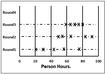
Step 5.2 − He then plots a chart on the whiteboard. He plots each member’s total project estimate as an X on the Round 1 line, without disclosing the corresponding names. The Estimation team gets an idea of the range of estimates, which initially may be large.

Step 5.3 − Each team member reads aloud the detailed task list that he/she made, identifying any assumptions made and raising any questions or issues. The task estimates are not disclosed.

The individual detailed task lists contribute to a more complete task list when combined.

Step 5.4 − The team then discusses any doubt/problem they have about the tasks they have arrived at, assumptions made, and estimation issues.

Step 5.5 − Each team member then revisits his/her task list and assumptions, and makes changes if necessary. The task estimates also may require adjustments based on the discussion, which are noted as +N Hrs. for more effort and –N Hrs. for less effort.

The team members then combine the changes in the task estimates to arrive at the total project estimate.

Step 5.6 − The moderator collects the changed estimates from all the team members and plots them on the Round 2 line.

In this round, the range will be narrower compared to the earlier one, as it is more consensus based.

Step 5.7 − The team then discusses the task modifications they have made and the assumptions.

Step 5.8 − Each team member then revisits his/her task list and assumptions, and makes changes if necessary. The task estimates may also require adjustments based on the discussion.

The team members then once again combine the changes in the task estimate to arrive at the total project estimate.

Step 5.9 − The moderator collects the changed estimates from all the members again and plots them on the Round 3 line.

Again, in this round, the range will be narrower compared to the earlier one.

Step 5.10 − Steps 5.7, 5.8, 5.9 are repeated till one of the following criteria is met −

• Results are converged to an acceptably narrow range.
• All team members are unwilling to change their latest estimates.
• The allotted Estimation meeting time is over.

Step 6 − The Project Manager then assembles the results from the Estimation meeting.

Step 6.1 − He compiles the individual task lists and the corresponding estimates into a single master task list.

Step 6.2 − He also combines the individual lists of assumptions.

Step 6.3 − He then reviews the final task list with the Estimation team.

Advantages and Disadvantages of Wideband Delphi Technique

Advantages

• Wideband Delphi Technique is a consensus-based estimation technique for estimating effort.
• Useful when estimating time to do a task.
• Participation of experienced people and they individually estimating would lead to reliable results.
• People who would do the work are making estimates thus making valid estimates.
• Anonymity maintained throughout makes it possible for everyone to express their results confidently.
• A very simple technique.
• Assumptions are documented, discussed and agreed.

Disadvantages

• Management support is required.
• The estimation results may not be what the management wants to hear.

Three-point Estimation looks at three values −

• the most optimistic estimate (O),
• a most likely estimate (M), and
• a pessimistic estimate (least likely estimate (L)).

There has been some confusion regarding Three-point Estimation and PERT in the industry. However, the techniques are different. You will see the differences as you learn the two techniques. Also, at the end of the PERT technique, the differences are collated and presented. If you want to look at them first, you can.

Three-point Estimate (E) is based on the simple average and follows triangular distribution.

E = (O + M + L) / 3

Standard Deviation

In Triangular Distribution,

Mean = (O + M + L) / 3

Standard Deviation = √ [((O − E)² + (M − E)² + (L − E)²) / 2]

Three-point Estimation Steps

Step 1 − Arrive at the WBS.

Step 2 − For each task, find three values − most optimistic estimate (O), a most likely estimate (M), and a pessimistic estimate (L).

Step 3 − Calculate the Mean of the three values.

Mean = (O + M + L) / 3

Step 4 − Calculate the Three-point Estimate of the task. Three-point Estimate is the Mean. Hence,

E = Mean = (O + M + L) / 3

Step 5 − Calculate the Standard Deviation of the task.

Standard Deviation (SD) = √ [((O − E)² + (M − E)² + (L - E)²)/2]

Step 6 − Repeat Steps 2, 3, 4 for all the Tasks in the WBS.

Step 7 − Calculate the Three-point Estimate of the project.

E (Project) = ∑ E (Task)

Step 8 − Calculate the Standard Deviation of the project.

SD (Project) = √ (∑SD (Task)²)

Convert the Project Estimates to Confidence Levels

The Three-point Estimate (E) and the Standard Deviation (SD) thus calculated are used to convert the project estimates to “Confidence Levels”.

The conversion is based such that −

• Confidence Level in E +/– SD is approximately 68%.
• Confidence Level in E value +/– 1.645 × SD is approximately 90%.
• Confidence Level in E value +/– 2 × SD is approximately 95%.
• Confidence Level in E value +/– 3 × SD is approximately 99.7%.

Commonly, the 95% Confidence Level, i.e., E Value + 2 × SD, is used for all project and task estimates.

Project Evaluation and Review Technique (PERT) estimation considers three values: the most optimistic estimate (O), a most likely estimate (M), and a pessimistic estimate (least likely estimate (L)). There has been some confusion regarding Three-point Estimation and PERT in the Industry. However, the techniques are different. You will see the differences as you learn the two techniques. Also, at the end of this chapter, the differences are collated and presented.

PERT is based on three values − most optimistic estimate (O), a most likely estimate (M), and a pessimistic estimate (least likely estimate (L)). The most-likely estimate is weighted 4 times more than the other two estimates (optimistic and pessimistic).

PERT Estimate (E) is based on the weighted average and follows beta distribution.

E = (O + 4 × M + L)/6

PERT is frequently used along with Critical Path Method (CPM). CPM tells about the tasks that are critical in the project. If there is a delay in these tasks, the project gets delayed.

Standard Deviation

Standard Deviation (SD) measures the variability or uncertainty in the estimate.

In beta distribution,

Mean = (O + 4 × M + L)/6

Standard Deviation (SD) = (L − O)/6

PERT Estimation Steps

Step (1) − Arrive at the WBS.

Step (2) − For each task, find three values most optimistic estimate (O), a most likely estimate (M), and a pessimistic estimate (L).

Step (3) − PERT Mean = (O + 4 × M + L)/6

PERT Mean = (O + 4 × M + L)/3

Step (4) − Calculate the Standard Deviation of the task.

Standard Deviation (SD) = (L − O)/6

Step (6) − Repeat steps 2, 3, 4 for all the tasks in the WBS.

Step (7) − Calculate the PERT estimate of the project.

E (Project) = ∑ E (Task)

Step (8) − Calculate the Standard Deviation of the project.

SD (Project) = √ (ΣSD (Task)²)

Convert the Project Estimates to Confidence Levels

PERT Estimate (E) and Standard Deviation (SD) thus calculated are used to convert the project estimates to confidence levels.

The conversion is based such that

• Confidence level in E +/– SD is approximately 68%.
• Confidence level in E value +/– 1.645 × SD is approximately 90%.
• Confidence level in E value +/– 2 × SD is approximately 95%.
• Confidence level in E value +/– 3 × SD is approximately 99.7%.

Commonly, the 95% confidence level, i.e., E Value + 2 × SD, is used for all project and task estimates.

Differences between Three-Point Estimation and PERT

Following are the differences between Three-Point Estimation and PERT −

Three-Point Estimation	PERT
Simple average	Weighted average
Follows triangular Distribution	Follows beta Distribution
Used for small repetitive projects	Used for large non-repetitive projects, usually R&D projects. Used along with Critical Path Method (CPM)
E = Mean = (O + M + L)/3 This is simple average	E = Mean = (O + 4 × M + L)/6 This is weighted average
SD = √ [((O − E)2 + (M − E)2 + (L − E)2)/2]	SD = (L − O)/6

Analogous Estimation uses a similar past project information to estimate the duration or cost of your current project, hence the word, "analogy". You can use analogous estimation when there is limited information regarding your current project.

Quite often, there will be situations when project managers will be asked to give cost and duration estimates for a new project as the executives need decision-making data to decide whether the project is worth doing. Usually, neither the project manager nor anyone else in the organization has ever done a project like the new one but the executives still want accurate cost and duration estimates.

In such cases, analogous estimation is the best solution. It may not be perfect but is accurate as it is based on past data. Analogous estimation is an easy-to-implement technique. The project success rate can be up to 60% as compared to the initial estimates.

Analogous Estimation – Definition

Analogous estimation is a technique which uses the values of parameters from historical data as the basis for estimating similar parameter for a future activity. Parameters examples: Scope, cost, and duration. Measures of scale examples − Size, weight, and complexity.

Because the project manager’s, and possibly the team’s experience and judgment are applied to the estimating process, it is considered a combination of historical information and expert judgment.

Analogous Estimation Requirements

For analogous estimation following is the requirement −

• Data from previous and on-going projects
  • Work hours per week of each team member
  • Costs involved to get the project completed
• Project close to the current project
• In case the current Project is new, and no past project is similar
  • Modules from past projects that are similar to those in current project
  • Activities from past projects that are similar to those in current project
  • Data from these selected ones
• Participation of the project manager and estimation team to ensure experienced judgment on the estimates.

Analogous Estimation Steps

The project manager and team have to collectively do analogous estimation.

• Step 1 − Identify the domain of the current project.

• Step 2 − Identify the technology of the current project.

• Step 3 − Look in the organization database if a similar project data is available. If available, go to Step (4). Otherwise go to Step (6).

• Step 4 − Compare the current project with the identified past project data.

• Step 5 − Arrive at the duration and cost estimates of the current project. This ends analogous estimation of the project.

• Step 6 − Look in the organization database if any past projects have similar modules as those in the current project.

• Step 7 − Look in the organization database if any past projects have similar activities as those in the current project.

• Step 8 − Collect all those and use expert judgment to arrive at the duration and cost estimates of the current project.

Advantages of Analogous Estimation

• Analogous estimation is a better way of estimation in the initial stages of the project when very few details are known.

• The technique is simple and time taken for estimation is very less.

• Organization’s success rate can be expected to be high since the technique is based on the organization’s past project data.

• Analogous estimation can be used to estimate the effort and duration of individual tasks too. Hence, in WBS when you estimate the tasks, you can use Analogy.

Work Breakdown Structure (WBS), in Project Management and Systems Engineering, is a deliverable-oriented decomposition of a project into smaller components. WBS is a key project deliverable that organizes the team's work into manageable sections. The Project Management Body of Knowledge (PMBOK) defines WBS as a "deliverable oriented hierarchical decomposition of the work to be executed by the project team."

WBS element may be a product, data, service, or any combination thereof. WBS also provides the necessary framework for detailed cost estimation and control along with providing guidance for schedule development and control.

Representation of WBS

WBS is represented as a hierarchical list of project’s work activities. There are two formats of WBS −

• Outline View (Indented Format)
• Tree Structure View (Organizational Chart)

Let us first discuss how to use the outline view for preparing a WBS.

Outline View

The outline view is a very user-friendly layout. It presents a good view of the entire project and allows easy modifications as well. It uses numbers to record the various stages of a project. It looks somewhat similar to the following −

• Software Development

• Scope

  • Determine project scope
  • Secure project sponsorship
  • Define preliminary resources
  • Secure core resources
  • Scope complete

• Analysis/Software Requirements

  • Conduct needs analysis
  • Draft preliminary software specifications
  • Develop preliminary budget
  • Review software specifications/budget with the team
  • Incorporate feedback on software specifications
  • Develop delivery timeline
  • Obtain approvals to proceed (concept, timeline, and budget)
  • Secure required resources
  • Analysis complete

• Design

  • Review preliminary software specifications
  • Develop functional specifications
  • Obtain approval to proceed
  • Design complete

• Development

  • Review functional specifications
  • Identify modular/tiered design parameters
  • Develop code
  • Developer testing (primary debugging)
  • Development complete

• Testing

  • Develop unit test plans using product specifications
  • Develop integration test plans using product specifications

• Training

  • Develop training specifications for end-users
  • Identify training delivery methodology (online, classroom, etc.)
  • Develop training materials
  • Finalize training materials
  • Develop training delivery mechanism
  • Training materials complete

• Deployment

  • Determine final deployment strategy
  • Develop deployment methodology
  • Secure deployment resources
  • Train support staff
  • Deploy software
  • Deployment complete

Let us now take a look at the tree structure view.

Tree Structure View

The Tree Structure View presents a very easy-to-understand view of the entire project. The following illustration shows how a tree structure view looks like. This type of organizational chart structure can be easily drawn with the features available in MS-Word.

Types of WBS

There are two types of WBS −

• Functional WBS − In functional WBS, the system is broken based on the functions in the application to be developed. This is useful in estimating the size of the system.

• Activity WBS − In activity WBS, the system is broken based on the activities in the system. The activities are further broken into tasks. This is useful in estimating effort and schedule in the system.

Estimate Size

Step 1 − Start with functional WBS.

Step 2 − Consider the leaf nodes.

Step 3 − Use either Analogy or Wideband Delphi to arrive at the size estimates.

Estimate Effort

Step 1 − Use Wideband Delphi Technique to construct WBS. We suggest that the tasks should not be more than 8 hrs. If a task is of larger duration, split it.

Step 2 − Use Wideband Delphi Technique or Three-point Estimation to arrive at the Effort Estimates for the Tasks.

Scheduling

Once the WBS is ready and the size and effort estimates are known, you are ready for scheduling the tasks.

While scheduling the tasks, certain things should be taken into account −

• Precedence − A task that must occur before another is said to have precedence of the other.

• Concurrence − Concurrent tasks are those that can occur at the same time (in parallel).

• Critical Path − Specific set of sequential tasks upon which the project completion date depends.

  • All projects have a critical path.
  • Accelerating non-critical tasks do not directly shorten the schedule.

Critical Path Method

Critical Path Method (CPM) is the process for determining and optimizing the critical path. Non-critical path tasks can start earlier or later without impacting the completion date.

Please note that critical path may change to another as you shorten the current one. For example, for WBS in the previous figure, the critical path would be as follows −

As the project completion date is based on a set of sequential tasks, these tasks are called critical tasks.

The project completion date is not based on the training, documentation and deployment. Such tasks are called non-critical tasks.

Task Dependency Relationships

Certain times, while scheduling, you may have to consider task dependency relationships. The important Task Dependency Relationships are −

• Finish-to-Start (FS)
• Finish-to-Finish (FF)

Finish-to-Start (FS)

In Finish-to-Start (FS) task dependency relationship, Task B cannot start till Task A is completed.

Finish-to-Finish (FF)

In Finish-to-Finish (FF) task dependency relationship, Task B cannot finish till Task A is completed.

Gantt Chart

A Gantt chart is a type of bar chart, adapted by Karol Adamiecki in 1896 and independently by Henry Gantt in the 1910s, that illustrates a project schedule. Gantt charts illustrate the start and finish dates of the terminal elements and summary elements of a project.

You can take the Outline Format in Figure 2 into Microsoft Project to obtain a Gantt Chart View.

Milestones

Milestones are the critical stages in your schedule. They will have a duration of zero and are used to flag that you have completed certain set of tasks. Milestones are usually shown as a diamond.

For example, in the above Gantt Chart, Design Complete and Development Complete are shown as milestones, represented with a diamond shape.

Milestones can be tied to Contract Terms.

Advantages of Estimation using WBS

WBS simplifies the process of project estimation to a great extent. It offers the following advantages over other estimation techniques −

• In WBS, the entire work to be done by the project is identified. Hence, by reviewing the WBS with project stakeholders, you will be less likely to omit any work needed to deliver the desired project deliverables.

• WBS results in more accurate cost and schedule estimates.

• The project manager obtains team participation to finalize the WBS. This involvement of the team generates enthusiasm and responsibility in the project.

• WBS provides a basis for task assignments. As a precise task is allocated to a particular team member who would be accountable for its accomplishment.

• WBS enables monitoring and controlling at task level. This allows you to measure progress and ensure that your project will be delivered on time.

Planning Poker Estimation

Planning Poker is a consensus-based technique for estimating, mostly used to estimate effort or relative size of user stories in Scrum.

Planning Poker combines three estimation techniques − Wideband Delphi Technique, Analogous Estimation, and Estimation using WBS.

Planning Poker was first defined and named by James Grenning in 2002 and later popularized by Mike Cohn in his book "Agile Estimating and Planning”, whose company trade marked the term.

Planning Poker Estimation Technique

In Planning Poker Estimation Technique, estimates for the user stories are derived by playing planning poker. The entire Scrum team is involved and it results in quick but reliable estimates.

• Planning Poker is played with a deck of cards. As Fibonacci sequence is used, the cards have numbers - 1, 2, 3, 5, 8, 13, 21, 34, etc. These numbers represent the “Story Points”. Each estimator has a deck of cards. The numbers on the cards should be large enough to be visible to all the team members, when one of the team members holds up a card.

• One of the team members is selected as the Moderator. The moderator reads the description of the user story for which estimation is being made. If the estimators have any questions, product owner answers them.

• Each estimator privately selects a card representing his or her estimate. Cards are not shown until all the estimators have made a selection. At that time, all cards are simultaneously turned over and held up so that all team members can see each estimate.

• In the first round, it is very likely that the estimations vary. The high and low estimators explain the reason for their estimates. Care should be taken that all the discussions are meant for understanding only and nothing is to be taken personally. The moderator has to ensure the same.

• The team can discuss the story and their estimates for a few more minutes.

• The moderator can take notes on the discussion that will be helpful when the specific story is developed. After the discussion, each estimator re-estimates by again selecting a card. Cards are once again kept private until everyone has estimated, at which point they are turned over at the same time.

Repeat the process till the estimates converge to a single estimate that can be used for the story. The number of rounds of estimation may vary from one user story to another.

Benefits of Planning Poker Estimation

Planning poker combines three methods of estimation −

Expert Opinion − In expert opinion-based estimation approach, an expert is asked how long something will take or how big it will be. The expert provides an estimate relying on his or her experience or intuition or gut feel. Expert Opinion Estimation usually doesn’t take much time and is more accurate compared to some of the analytical methods.

Analogy − Analogy estimation uses comparison of user stories. The user story under estimation is compared with similar user stories implemented earlier, giving accurate results as the estimation is based on proven data.

Disaggregation − Disaggregation estimation is done by splitting a user story into smaller, easier-to-estimate user stories. The user stories to be included in a sprint are normally in the range of two to five days to develop. Hence, the user stories that possibly take longer duration need to be split into smaller use-Cases. This approach also ensures that there would be many stories that are comparable.

Test efforts are not based on any definitive timeframe. The efforts continue until some pre-decided timeline is set, irrespective of the completion of testing.

This is mostly due to the fact that conventionally, test effort estimation is a part of the development estimation. Only in the case of estimation techniques that use WBS, such as Wideband Delphi, Three-point Estimation, PERT, and WBS, you can obtain the values for the estimates of the testing activities.

If you have obtained the estimates as Function Points (FP), then as per Caper Jones,

Number of Test Cases = (Number of Function Points) × 1.2

Once you have the number of test cases, you can take productivity data from organizational database and arrive at the effort required for testing.

Percentage of Development Effort Method

Test effort required is a direct proportionate or percentage of the development effort. Development effort can be estimated using Lines of Code (LOC) or Function Points (FP). Then, the percentage of effort for testing is obtained from Organization Database. The percentage so obtained is used to arrive at the effort estimate for testing.

Estimating Testing Projects

Several organizations are now providing independent verification and validation services to their clients and that would mean the project activities would entirely be testing activities.

Estimating testing projects requires experience on varied projects for the software test life cycle. When you are estimating a testing project, consider −

• Team skills
• Domain Knowledge
• Complexity of the application
• Historical data
• Bug cycles for the project
• Resources availability
• Productivity variations
• System environment and downtime

Testing Estimation Techniques

The following testing estimation techniques are proven to be accurate and are widely used −

• PERT software testing estimation technique
• UCP Method
• WBS
• Wideband Delphi technique
• Function point/Testing point analysis
• Percentage distribution
• Experience-based testing estimation technique

PERT Software Testing Estimation Technique

PERT software testing estimation technique is based on statistical methods in which each testing task is broken down into sub-tasks and then three types of estimation are done on each sub-tasks.

The formula used by this technique is −

Test Estimate = (O + (4 × M) + E)/6

Where,

O = Optimistic estimate (best case scenario in which nothing goes wrong and all conditions are optimal).

M = Most likely estimate (most likely duration and there may be some problem but most of the things will go right).

L = Pessimistic estimate (worst case scenario where everything goes wrong).

Standard Deviation for the technique is calculated as −

Standard Deviation (SD) = (E − O)/6

Use-Case Point Method

UCP Method is based on the use cases where we calculate the unadjusted actor weights and unadjusted use case weights to determine the software testing estimation.

Use-case is a document which specifies different users, systems or other stakeholders interacting with the concerned application. They are named as “Actors”. The interactions accomplish some defined goals protecting the interest of all stakeholders through different behavior or flow termed as scenarios.

Step 1 − Count the no. of actors. Actors include positive, negative and exceptional.

Step 2 − Calculate unadjusted actor weights as

Unadjusted Actor Weights = Total no. of Actors

Step 3 − Count the number of use-cases.

Step 4 − Calculate unadjusted use-case weights as

Unadjusted Use-Case Weights = Total no. of Use-Cases

Step 5 − Calculate unadjusted use-case points as

Unadjusted Use-Case Points = (Unadjusted Actor Weights + Unadjusted Use-Case Weights)

Step 6 − Determine the technical/environmental factor (TEF). If unavailable, take it as 0.50.

Step 7 − Calculate adjusted use-case point as

Adjusted Use-Case Point = Unadjusted Use-Case Points × [0.65 + (0.01 × TEF]

Step 8 − Calculate total effort as

Total Effort = Adjusted Use-Case Point × 2

Work Breakdown Structure

Step 1 − Create WBS by breaking down the test project into small pieces.

Step 2 − Divide modules into sub-modules.

Step 3 Divide sub-modules further into functionalities.

Step 4 − Divide functionalities into sub-functionalities.

Step 5 − Review all the testing requirements to make sure they are added in WBS.

Step 6 − Figure out the number of tasks your team needs to complete.

Step 7 − Estimate the effort for each task.

Step 8 − Estimate the duration of each task.

Wideband Delphi Technique

In Wideband Delphi Method, WBS is distributed to a team comprising of 3-7 members for re-estimating the tasks. The final estimate is the result of the summarized estimates based on the team consensus.

This method speaks more on experience rather than any statistical formula. This method was popularized by Barry Boehm to emphasize on the group iteration to reach a consensus where the team visualized different aspects of the problems while estimating the test effort.

Function Point / Testing Point Analysis

FPs indicate the functionality of software application from the user's perspective and is used as a technique to estimate the size of a software project.

In testing, estimation is based on requirement specification document, or on a previously created prototype of the application. To calculate FP for a project, some major components are required. They are −

• Unadjusted Data Function Points − i) Internal Files, ii) External Interfaces

• Unadjusted Transaction Function Points − i) User Inputs, ii) User Outputs & iii) User Inquiries

• Capers Jones basic formula −

  Number of Test Cases = (Number of Function Points) × 1.2

• Total Actual Effort (TAE) −

  (Number of Test cases) × (Percentage of Development Effort /100)

Percentage Distribution

In this technique, all the phases of Software Development Life Cycle (SDLC) are assigned effort in %. This can be based on past data from similar projects. For example −

Phase	% of Effort
Project Management	7%
Requirements	9%
Design	16%
Coding	26%
Testing (all Test Phases)	27%
Documentation	9%
Installation and Training	6%

Next, % of effort for testing (all test phases) is further distributed for all Testing Phases −

All Testing Phases	% of Effort
Component Testing	16
Independent Testing	84
Total	100

Independent Testing	% of Effort
Integration Testing	24
System Testing	52
Acceptance Testing	24
Total	100

System Testing	% of Effort
Functional System Testing	65
Non-functional System Testing	35
Total	100

Test Planning and Design Architecture	50%
Review phase	50%

Experience-based Testing Estimation Technique

This technique is based on analogies and experts. The technique assumes that you already tested similar applications in previous projects and collected metrics from those projects. You also collected metrics from previous tests. Take inputs from subject matter experts who know the application (as well as testing) very well and use the metrics you have collected and arrive at the testing effort.