Microsoft Cognitive Toolkit - Guida rapida
In questo capitolo impareremo cos'è CNTK, le sue caratteristiche, la differenza tra la sua versione 1.0 e 2.0 e gli importanti punti salienti della versione 2.7.
Che cos'è Microsoft Cognitive Toolkit (CNTK)?
Microsoft Cognitive Toolkit (CNTK), precedentemente noto come Computational Network Toolkit, è un toolkit gratuito, di facile utilizzo, open source e di livello commerciale che ci consente di addestrare algoritmi di deep learning per apprendere come il cervello umano. Ci consente di creare alcuni popolari sistemi di apprendimento profondo comefeed-forward neural network time series prediction systems and Convolutional neural network (CNN) image classifiers.
Per prestazioni ottimali, le sue funzioni del framework sono scritte in C ++. Sebbene possiamo chiamare la sua funzione usando C ++, ma l'approccio più comunemente usato per lo stesso è usare un programma Python.
Caratteristiche di CNTK
Di seguito sono riportate alcune delle caratteristiche e delle capacità offerte nell'ultima versione di Microsoft CNTK:
Componenti incorporati
CNTK ha componenti integrati altamente ottimizzati in grado di gestire dati multidimensionali densi o sparsi da Python, C ++ o BrainScript.
Possiamo implementare CNN, FNN, RNN, Batch Normalization e Sequence-to-Sequence con attenzione.
Ci fornisce la funzionalità per aggiungere nuovi componenti core definiti dall'utente sulla GPU da Python.
Fornisce inoltre l'ottimizzazione automatica degli iperparametri.
Possiamo implementare l'apprendimento per rinforzo, le reti generative antagoniste (GAN), l'apprendimento supervisionato e non supervisionato.
Per enormi set di dati, CNTK dispone di lettori ottimizzati incorporati.
Utilizzo efficiente delle risorse
CNTK ci fornisce parallelismo con elevata precisione su più GPU / macchine tramite SGD a 1 bit.
Per adattarsi ai modelli più grandi nella memoria della GPU, fornisce la condivisione della memoria e altri metodi integrati.
Esprimi facilmente le nostre reti
CNTK dispone di API complete per la definizione della propria rete, studenti, lettori, formazione e valutazione da Python, C ++ e BrainScript.
Usando CNTK, possiamo facilmente valutare modelli con Python, C ++, C # o BrainScript.
Fornisce API sia di alto livello che di basso livello.
Sulla base dei nostri dati, può modellare automaticamente l'inferenza.
Ha loop simbolici Recurrent Neural Network (RNN) completamente ottimizzati.
Misurazione delle prestazioni del modello
CNTK fornisce vari componenti per misurare le prestazioni delle reti neurali create.
Genera dati di registro dal tuo modello e dall'ottimizzatore associato, che possiamo utilizzare per monitorare il processo di addestramento.
Versione 1.0 vs Versione 2.0
La tabella seguente confronta CNTK versione 1.0 e 2.0:
| Versione 1.0.0 | Versione 2.0 |
|---|---|
| È stato rilasciato nel 2016. | Si tratta di una riscrittura significativa della versione 1.0 ed è stata rilasciata a giugno 2017. |
| Utilizzava un linguaggio di scripting proprietario chiamato BrainScript. | Le sue funzioni di framework possono essere chiamate usando C ++, Python. Possiamo facilmente caricare i nostri moduli in C # o Java. BrainScript è supportato anche dalla versione 2.0. |
| Funziona su entrambi i sistemi Windows e Linux ma non direttamente su Mac OS. | Funziona anche su sistemi Windows (Win 8.1, Win 10, Server 2012 R2 e versioni successive) e Linux, ma non direttamente su Mac OS. |
Punti salienti importanti della versione 2.7
Version 2.7è l'ultima versione principale rilasciata di Microsoft Cognitive Toolkit. Ha pieno supporto per ONNX 1.4.1. Di seguito sono riportati alcuni importanti punti salienti di quest'ultima versione rilasciata di CNTK.
Supporto completo per ONNX 1.4.1.
Supporto per CUDA 10 per sistemi Windows e Linux.
Supporta il ciclo avanzato RNN (Recurrent Neural Networks) nell'esportazione ONNX.
Può esportare più di 2 GB di modelli in formato ONNX.
Supporta FP16 nell'azione di addestramento del linguaggio di scripting BrainScript.
Qui, capiremo l'installazione di CNTK su Windows e su Linux. Inoltre, il capitolo spiega l'installazione del pacchetto CNTK, i passaggi per installare Anaconda, i file CNTK, la struttura delle directory e l'organizzazione della libreria CNTK.
Prerequisiti
Per installare CNTK, dobbiamo avere Python installato sui nostri computer. Puoi andare al linkhttps://www.python.org/downloads/e seleziona l'ultima versione per il tuo sistema operativo, ovvero Windows e Linux / Unix. Per il tutorial di base su Python, puoi fare riferimento al linkhttps://www.tutorialspoint.com/python3/index.htm.

CNTK è supportato sia per Windows che per Linux, quindi li esamineremo entrambi.
Installazione su Windows
Per eseguire CNTK su Windows, utilizzeremo il Anaconda versiondi Python. Lo sappiamo, Anaconda è una ridistribuzione di Python. Include pacchetti aggiuntivi comeScipy eScikit-learn che vengono utilizzati da CNTK per eseguire vari calcoli utili.
Quindi, prima vediamo i passaggi per installare Anaconda sulla tua macchina -
Step 1−Prima scarica i file di installazione dal sito web pubblico https://www.anaconda.com/distribution/.
Step 2 - Una volta scaricati i file di installazione, avvia l'installazione e segui le istruzioni dal link https://docs.anaconda.com/anaconda/install/.
Step 3- Una volta installato, Anaconda installerà anche altre utilità, che includeranno automaticamente tutti gli eseguibili di Anaconda nella variabile PATH del tuo computer. Possiamo gestire il nostro ambiente Python da questo prompt, possiamo installare pacchetti ed eseguire script Python.
Installazione del pacchetto CNTK
Una volta completata l'installazione di Anaconda, è possibile utilizzare il modo più comune per installare il pacchetto CNTK tramite l'eseguibile pip utilizzando il seguente comando:
pip install cntkEsistono vari altri metodi per installare Cognitive Toolkit sulla macchina. Microsoft ha un set accurato di documentazione che spiega in dettaglio gli altri metodi di installazione. Segui il linkhttps://docs.microsoft.com/en-us/cognitive-toolkit/Setup-CNTK-on-your-machine.
Installazione su Linux
L'installazione di CNTK su Linux è leggermente diversa dalla sua installazione su Windows. Qui, per Linux useremo Anaconda per installare CNTK, ma invece di un programma di installazione grafico per Anaconda, useremo un programma di installazione basato su terminale su Linux. Sebbene il programma di installazione funzioni con quasi tutte le distribuzioni Linux, abbiamo limitato la descrizione a Ubuntu.
Quindi, prima vediamo i passaggi per installare Anaconda sulla tua macchina -
Passaggi per installare Anaconda
Step 1- Prima di installare Anaconda, assicurati che il sistema sia completamente aggiornato. Per verificare, eseguire prima i seguenti due comandi all'interno di un terminale:
sudo apt update
sudo apt upgrade
Step 2 - Una volta aggiornato il computer, ottieni l'URL dal sito web pubblico https://www.anaconda.com/distribution/ per gli ultimi file di installazione di Anaconda.
Step 3 - Una volta che l'URL è stato copiato, apri una finestra di terminale ed esegui il seguente comando:
wget -0 anaconda-installer.sh url SHAPE \* MERGEFORMAT
     y


	             f


      x

|                     }
Sostituisci il url segnaposto con l'URL copiato dal sito Anaconda.
Step 4 - Successivamente, con l'aiuto del seguente comando, possiamo installare Anaconda -
sh ./anaconda-installer.shIl comando precedente verrà installato per impostazione predefinita Anaconda3 all'interno della nostra home directory.
Installazione del pacchetto CNTK
Una volta completata l'installazione di Anaconda, è possibile utilizzare il modo più comune per installare il pacchetto CNTK tramite l'eseguibile pip utilizzando il seguente comando:
pip install cntkEsame dei file CNTK e della struttura delle directory
Una volta installato CNTK come pacchetto Python, possiamo esaminarne la struttura di file e directory. È aC:\Users\

Verifica dell'installazione di CNTK
Una volta installato CNTK come pacchetto Python, è necessario verificare che CNTK sia stato installato correttamente. Dalla shell dei comandi di Anaconda, avvia l'interprete Python inserendoipython. Quindi, importa CNTK inserendo il seguente comando.
import cntk as cUna volta importato, controlla la sua versione con l'aiuto del seguente comando:
print(c.__version__)L'interprete risponderà con la versione CNTK installata. Se non risponde, ci sarà un problema con l'installazione.
L'organizzazione della biblioteca CNTK
CNTK, tecnicamente un pacchetto python, è organizzato in 13 sotto-pacchetti di alto livello e 8 sotto-pacchetti più piccoli. La seguente tabella è composta dai 10 pacchetti più utilizzati:
| Suor n | Nome e descrizione del pacchetto |
|---|---|
| 1 | cntk.io Contiene funzioni per la lettura dei dati. Ad esempio: next_minibatch () |
| 2 | cntk.layers Contiene funzioni di alto livello per la creazione di reti neurali. Ad esempio: Dense () |
| 3 | cntk.learners Contiene funzioni per l'addestramento. Ad esempio: sgd () |
| 4 | cntk.losses Contiene funzioni per misurare l'errore di addestramento. Ad esempio: squared_error () |
| 5 | cntk.metrics Contiene funzioni per misurare l'errore del modello. Ad esempio: classificatoin_error |
| 6 | cntk.ops Contiene funzioni di basso livello per la creazione di reti neurali. Ad esempio: tanh () |
| 7 | cntk.random Contiene funzioni per generare numeri casuali. Ad esempio: normal () |
| 8 | cntk.train Contiene funzioni di allenamento. Ad esempio: train_minibatch () |
| 9 | cntk.initializer Contiene inizializzatori di parametri del modello. Ad esempio: normal () e uniform () |
| 10 | cntk.variables Contiene costrutti di basso livello. Ad esempio: Parameter () e Variable () |
Microsoft Cognitive Toolkit offre due diverse versioni di build, ovvero solo CPU e solo GPU.
Versione build solo CPU
La versione build solo CPU di CNTK utilizza Intel MKLML ottimizzato, dove MKLML è il sottoinsieme di MKL (Math Kernel Library) e rilasciato con Intel MKL-DNN come versione terminata di Intel MKL per MKL-DNN.
Versione build solo GPU
D'altra parte, la versione build solo GPU di CNTK utilizza librerie NVIDIA altamente ottimizzate come CUB e cuDNN. Supporta la formazione distribuita su più GPU e più macchine. Per una formazione distribuita ancora più veloce in CNTK, la versione GPU-build include anche:
SGD quantizzato a 1 bit sviluppato da MSR.
Algoritmi di formazione parallela SGD block-momentum.
Abilitazione della GPU con CNTK su Windows
Nella sezione precedente abbiamo visto come installare la versione base di CNTK da utilizzare con la CPU. Ora parliamo di come possiamo installare CNTK da utilizzare con una GPU. Ma, prima di approfondire la questione, prima dovresti avere una scheda grafica supportata.
Al momento, CNTK supporta la scheda grafica NVIDIA con supporto almeno CUDA 3.0. Per essere sicuro, puoi controllare ahttps://developer.nvidia.com/cuda-gpus se la tua GPU supporta CUDA.
Quindi, vediamo i passaggi per abilitare la GPU con CNTK su sistema operativo Windows -
Step 1 - A seconda della scheda grafica che stai utilizzando, devi prima disporre dei driver GeForce o Quadro più recenti per la tua scheda grafica.
Step 2 - Dopo aver scaricato i driver, è necessario installare il toolkit CUDA versione 9.0 per Windows dal sito Web di NVIDIA https://developer.nvidia.com/cuda-90-download-archive?target_os=Windows&target_arch=x86_64. Dopo l'installazione, esegui il programma di installazione e segui le istruzioni.
Step 3 - Successivamente, è necessario installare i binari cuDNN dal sito Web di NVIDIA https://developer.nvidia.com/rdp/form/cudnn-download-survey. Con la versione CUDA 9.0, cuDNN 7.4.1 funziona bene. Fondamentalmente, cuDNN è uno strato nella parte superiore di CUDA, utilizzato da CNTK.
Step 4 - Dopo aver scaricato i file binari cuDNN, è necessario estrarre il file zip nella cartella principale dell'installazione del toolkit CUDA.
Step 5- Questo è l'ultimo passaggio che consentirà l'utilizzo della GPU all'interno di CNTK. Esegui il seguente comando all'interno del prompt di Anaconda su sistema operativo Windows -
pip install cntk-gpuAbilitazione della GPU con CNTK su Linux
Vediamo come possiamo abilitare la GPU con CNTK su sistema operativo Linux -
Download del toolkit CUDA
Innanzitutto, è necessario installare il toolkit CUDA dal sito Web NVIDIA https://developer.nvidia.com/cuda-90-download-archive?target_os=Linux&target_arch=x86_64&target_distro=Ubuntu&target_version=1604&target_type = runfilelocal .
Esecuzione del programma di installazione
Ora, una volta che hai i binari sul disco, esegui il programma di installazione aprendo un terminale ed eseguendo il seguente comando e le istruzioni sullo schermo:
sh cuda_9.0.176_384.81_linux-runModifica lo script del profilo Bash
Dopo aver installato il toolkit CUDA sulla tua macchina Linux, devi modificare lo script del profilo BASH. Per questo, prima apri il file $ HOME / .bashrc nell'editor di testo. Ora, alla fine dello script, includi le seguenti righe:
export PATH=/usr/local/cuda-9.0/bin${PATH:+:${PATH}} export LD_LIBRARY_PATH=/usr/local/cuda-9.0/lib64\ ${LD_LIBRARY_PATH:+:${LD_LIBRARY_PATH}}
Installing
Installazione delle librerie cuDNN
Alla fine dobbiamo installare i binari cuDNN. Può essere scaricato dal sito Web NVIDIAhttps://developer.nvidia.com/rdp/form/cudnn-download-survey. Con la versione CUDA 9.0, cuDNN 7.4.1 funziona bene. Fondamentalmente, cuDNN è uno strato nella parte superiore di CUDA, utilizzato da CNTK.
Una volta scaricata la versione per Linux, estraila nel file /usr/local/cuda-9.0 cartella utilizzando il seguente comando:
tar xvzf -C /usr/local/cuda-9.0/ cudnn-9.0-linux-x64-v7.4.1.5.tgzModificare il percorso del nome del file come richiesto.
In questo capitolo impareremo in dettaglio le sequenze in CNTK e la sua classificazione.
Tensori
Il concetto su cui lavora CNTK è tensor. Fondamentalmente, gli input, gli output ei parametri CNTK sono organizzati come filetensors, che è spesso pensato come una matrice generalizzata. Ogni tensore ha un'estensionerank -
Il tensore di rango 0 è uno scalare.
Il tensore di rango 1 è un vettore.
Il tensore di rango 2 è una matrice.
Qui, queste diverse dimensioni sono indicate come axes.
Assi statici e assi dinamici
Come suggerisce il nome, gli assi statici hanno la stessa lunghezza per tutta la vita della rete. D'altra parte, la lunghezza degli assi dinamici può variare da istanza a istanza. In effetti, la loro lunghezza in genere non è nota prima che venga presentato ogni minibatch.
Gli assi dinamici sono come gli assi statici perché definiscono anche un raggruppamento significativo dei numeri contenuti nel tensore.
Esempio
Per renderlo più chiaro, vediamo come viene rappresentato in CNTK un minibatch di brevi video clip. Supponiamo che la risoluzione dei video clip sia tutta 640 * 480. Inoltre, anche i clip vengono ripresi a colori, che è tipicamente codificato con tre canali. Significa inoltre che il nostro minibatch ha quanto segue:
3 assi statici di lunghezza 640, 480 e 3 rispettivamente.
Due assi dinamici; la lunghezza del video e gli assi del minibatch.
Significa che se un minibatch ha 16 video ciascuno dei quali è lungo 240 fotogrammi, sarebbe rappresentato come 16*240*3*640*480 tensori.
Lavorare con sequenze in CNTK
Cerchiamo di comprendere le sequenze in CNTK imparando prima la rete di memoria a lungo termine.
Rete di memoria a lungo termine (LSTM)

Le reti di memoria a lungo termine (LSTM) sono state introdotte da Hochreiter & Schmidhuber. Ha risolto il problema di ottenere un livello ricorrente di base per ricordare le cose per molto tempo. L'architettura di LSTM è data sopra nel diagramma. Come possiamo vedere, ha neuroni di input, celle di memoria e neuroni di output. Per combattere il problema del gradiente di fuga, le reti di memoria a lungo termine utilizzano una cella di memoria esplicita (memorizza i valori precedenti) e le seguenti porte:
Forget gate- Come suggerisce il nome, dice alla cella di memoria di dimenticare i valori precedenti. La cella di memoria memorizza i valori fino a quando il gate, ovvero "dimentica porta", gli dice di dimenticarli.
Input gate - Come suggerisce il nome, aggiunge nuove cose alla cella.
Output gate - Come suggerisce il nome, la porta di uscita decide quando passare lungo i vettori dalla cella al successivo stato nascosto.
È molto facile lavorare con le sequenze in CNTK. Vediamolo con l'aiuto del seguente esempio:
import sys
import os
from cntk import Trainer, Axis
from cntk.io import MinibatchSource, CTFDeserializer, StreamDef, StreamDefs,\
   INFINITELY_REPEAT
from cntk.learners import sgd, learning_parameter_schedule_per_sample
from cntk import input_variable, cross_entropy_with_softmax, \
   classification_error, sequence
from cntk.logging import ProgressPrinter
from cntk.layers import Sequential, Embedding, Recurrence, LSTM, Dense
def create_reader(path, is_training, input_dim, label_dim):
   return MinibatchSource(CTFDeserializer(path, StreamDefs(
      features=StreamDef(field='x', shape=input_dim, is_sparse=True),
      labels=StreamDef(field='y', shape=label_dim, is_sparse=False)
   )), randomize=is_training,
   max_sweeps=INFINITELY_REPEAT if is_training else 1)
def LSTM_sequence_classifier_net(input, num_output_classes, embedding_dim,
LSTM_dim, cell_dim):
   lstm_classifier = Sequential([Embedding(embedding_dim),
      Recurrence(LSTM(LSTM_dim, cell_dim)),
      sequence.last,
      Dense(num_output_classes)])
return lstm_classifier(input)
def train_sequence_classifier():
   input_dim = 2000
   cell_dim = 25
   hidden_dim = 25
   embedding_dim = 50
   num_output_classes = 5
   features = sequence.input_variable(shape=input_dim, is_sparse=True)
   label = input_variable(num_output_classes)
   classifier_output = LSTM_sequence_classifier_net(
   features, num_output_classes, embedding_dim, hidden_dim, cell_dim)
   ce = cross_entropy_with_softmax(classifier_output, label)
   pe =      classification_error(classifier_output, label)
   rel_path = ("../../../Tests/EndToEndTests/Text/" +
      "SequenceClassification/Data/Train.ctf")
   path = os.path.join(os.path.dirname(os.path.abspath(__file__)), rel_path)
   reader = create_reader(path, True, input_dim, num_output_classes)
input_map = {
   features: reader.streams.features,
   label: reader.streams.labels
}
lr_per_sample = learning_parameter_schedule_per_sample(0.0005)
progress_printer = ProgressPrinter(0)
trainer = Trainer(classifier_output, (ce, pe),
sgd(classifier_output.parameters, lr=lr_per_sample),progress_printer)
minibatch_size = 200
for i in range(255):
   mb = reader.next_minibatch(minibatch_size, input_map=input_map)
trainer.train_minibatch(mb)
   evaluation_average = float(trainer.previous_minibatch_evaluation_average)
   loss_average = float(trainer.previous_minibatch_loss_average)
return evaluation_average, loss_average
if __name__ == '__main__':
   error, _ = train_sequence_classifier()
   print(" error: %f" % error)
average since average since examples
loss last metric last
------------------------------------------------------
1.61 1.61 0.886 0.886 44
1.61 1.6 0.714 0.629 133
1.6 1.59 0.56 0.448 316
1.57 1.55 0.479 0.41 682
1.53 1.5 0.464 0.449 1379
1.46 1.4 0.453 0.441 2813
1.37 1.28 0.45 0.447 5679
1.3 1.23 0.448 0.447 11365
error: 0.333333La spiegazione dettagliata del programma di cui sopra sarà trattata nelle prossime sezioni, specialmente quando costruiremo reti neurali ricorrenti.
Questo capitolo tratta della costruzione di un modello di regressione logistica in CNTK.
Nozioni di base sul modello di regressione logistica
La regressione logistica, una delle tecniche ML più semplici, è una tecnica specifica per la classificazione binaria. In altre parole, per creare un modello di previsione in situazioni in cui il valore della variabile da prevedere può essere uno dei due soli valori categoriali. Uno degli esempi più semplici di regressione logistica è prevedere se la persona è maschio o femmina, in base all'età, alla voce, ai capelli e così via della persona.
Esempio
Comprendiamo matematicamente il concetto di regressione logistica con l'aiuto di un altro esempio:
Supponiamo di voler prevedere l'affidabilità creditizia di una richiesta di prestito; 0 significa rifiutare e 1 significa approvare, in base al richiedentedebt , income e credit rating. Rappresentiamo debito con X1, reddito con X2 e rating del credito con X3.
In Regressione logistica, determiniamo un valore di peso, rappresentato da w, per ogni caratteristica e un singolo valore di polarizzazione, rappresentato da b.
Ora supponiamo,
X1 = 3.0
X2 = -2.0
X3 = 1.0
E supponiamo di determinare il peso e il bias come segue:
W1 = 0.65, W2 = 1.75, W3 = 2.05 and b = 0.33Ora, per prevedere la classe, dobbiamo applicare la seguente formula:
Z = (X1*W1)+(X2*W2)+(X3+W3)+b
i.e. Z = (3.0)*(0.65) + (-2.0)*(1.75) + (1.0)*(2.05) + 0.33
= 0.83
Successivamente, dobbiamo calcolare P = 1.0/(1.0 + exp(-Z)). Qui, la funzione exp () è il numero di Eulero.
P = 1.0/(1.0 + exp(-0.83)
= 0.6963
Il valore P può essere interpretato come la probabilità che la classe sia 1. Se P <0,5, la previsione è classe = 0 altrimenti la previsione (P> = 0,5) è classe = 1.
Per determinare i valori di peso e bias, è necessario ottenere una serie di dati di addestramento con i valori predittori di input noti e i valori delle etichette di classe corretti noti. Dopodiché, possiamo utilizzare un algoritmo, generalmente Gradient Descent, per trovare i valori di peso e bias.
Esempio di implementazione del modello LR
Per questo modello LR, utilizzeremo il seguente set di dati:
1.0, 2.0, 0
3.0, 4.0, 0
5.0, 2.0, 0
6.0, 3.0, 0
8.0, 1.0, 0
9.0, 2.0, 0
1.0, 4.0, 1
2.0, 5.0, 1
4.0, 6.0, 1
6.0, 5.0, 1
7.0, 3.0, 1
8.0, 5.0, 1
Per avviare l'implementazione del modello LR in CNTK, dobbiamo prima importare i seguenti pacchetti:
import numpy as np
import cntk as C
Il programma è strutturato con la funzione main () come segue:
def main():
print("Using CNTK version = " + str(C.__version__) + "\n")
Ora, dobbiamo caricare i dati di allenamento in memoria come segue:
data_file = ".\\dataLRmodel.txt"
print("Loading data from " + data_file + "\n")
features_mat = np.loadtxt(data_file, dtype=np.float32, delimiter=",", skiprows=0, usecols=[0,1])
labels_mat = np.loadtxt(data_file, dtype=np.float32, delimiter=",", skiprows=0, usecols=[2], ndmin=2)
Ora creeremo un programma di addestramento che crei un modello di regressione logistica compatibile con i dati di addestramento -
features_dim = 2
labels_dim = 1
X = C.ops.input_variable(features_dim, np.float32)
y = C.input_variable(labels_dim, np.float32)
W = C.parameter(shape=(features_dim, 1)) # trainable cntk.Parameter
b = C.parameter(shape=(labels_dim))
z = C.times(X, W) + b
p = 1.0 / (1.0 + C.exp(-z))
model = p
Ora, dobbiamo creare Lerner e il trainer come segue:
ce_error = C.binary_cross_entropy(model, y) # CE a bit more principled for LR
fixed_lr = 0.010
learner = C.sgd(model.parameters, fixed_lr)
trainer = C.Trainer(model, (ce_error), [learner])
max_iterations = 4000
Formazione modello LR
Dopo aver creato il modello LR, è ora di iniziare il processo di formazione:
np.random.seed(4)
N = len(features_mat)
for i in range(0, max_iterations):
row = np.random.choice(N,1) # pick a random row from training items
trainer.train_minibatch({ X: features_mat[row], y: labels_mat[row] })
if i % 1000 == 0 and i > 0:
mcee = trainer.previous_minibatch_loss_average
print(str(i) + " Cross-entropy error on curr item = %0.4f " % mcee)
Ora, con l'aiuto del codice seguente, possiamo stampare i pesi e il bias del modello:
np.set_printoptions(precision=4, suppress=True)
print("Model weights: ")
print(W.value)
print("Model bias:")
print(b.value)
print("")
if __name__ == "__main__":
main()
Addestramento di un modello di regressione logistica - Esempio completo
import numpy as np
import cntk as C
   def main():
print("Using CNTK version = " + str(C.__version__) + "\n")
data_file = ".\\dataLRmodel.txt" # provide the name and the location of data file
print("Loading data from " + data_file + "\n")
features_mat = np.loadtxt(data_file, dtype=np.float32, delimiter=",", skiprows=0, usecols=[0,1])
labels_mat = np.loadtxt(data_file, dtype=np.float32, delimiter=",", skiprows=0, usecols=[2], ndmin=2)
features_dim = 2
labels_dim = 1
X = C.ops.input_variable(features_dim, np.float32)
y = C.input_variable(labels_dim, np.float32)
W = C.parameter(shape=(features_dim, 1)) # trainable cntk.Parameter
b = C.parameter(shape=(labels_dim))
z = C.times(X, W) + b
p = 1.0 / (1.0 + C.exp(-z))
model = p
ce_error = C.binary_cross_entropy(model, y) # CE a bit more principled for LR
fixed_lr = 0.010
learner = C.sgd(model.parameters, fixed_lr)
trainer = C.Trainer(model, (ce_error), [learner])
max_iterations = 4000
np.random.seed(4)
N = len(features_mat)
for i in range(0, max_iterations):
row = np.random.choice(N,1) # pick a random row from training items
trainer.train_minibatch({ X: features_mat[row], y: labels_mat[row] })
if i % 1000 == 0 and i > 0:
mcee = trainer.previous_minibatch_loss_average
print(str(i) + " Cross-entropy error on curr item = %0.4f " % mcee)
np.set_printoptions(precision=4, suppress=True)
print("Model weights: ")
print(W.value)
print("Model bias:")
print(b.value)
if __name__ == "__main__":
  main()
Produzione
Using CNTK version = 2.7
1000 cross entropy error on curr item = 0.1941
2000 cross entropy error on curr item = 0.1746
3000 cross entropy error on curr item = 0.0563
Model weights:
[-0.2049]
   [0.9666]]
Model bias:
[-2.2846]
Previsione utilizzando il modello LR addestrato
Una volta che il modello LR è stato addestrato, possiamo usarlo per la previsione come segue:
Prima di tutto, il nostro programma di valutazione importa il pacchetto numpy e carica i dati di addestramento in una matrice di caratteristiche e una matrice di etichette di classe nello stesso modo del programma di addestramento che implementiamo sopra -
import numpy as np
def main():
data_file = ".\\dataLRmodel.txt" # provide the name and the location of data file
features_mat = np.loadtxt(data_file, dtype=np.float32, delimiter=",",
skiprows=0, usecols=(0,1))
labels_mat = np.loadtxt(data_file, dtype=np.float32, delimiter=",",
skiprows=0, usecols=[2], ndmin=2)
Successivamente, è il momento di impostare i valori dei pesi e il bias che sono stati determinati dal nostro programma di allenamento -
print("Setting weights and bias values \n")
weights = np.array([0.0925, 1.1722], dtype=np.float32)
bias = np.array([-4.5400], dtype=np.float32)
N = len(features_mat)
features_dim = 2
Successivamente il nostro programma di valutazione calcolerà la probabilità di regressione logistica esaminando ogni elemento di formazione come segue:
print("item pred_prob pred_label act_label result")
for i in range(0, N): # each item
   x = features_mat[i]
   z = 0.0
   for j in range(0, features_dim):
   z += x[j] * weights[j]
   z += bias[0]
   pred_prob = 1.0 / (1.0 + np.exp(-z))
  pred_label = 0 if pred_prob < 0.5 else 1
   act_label = labels_mat[i]
   pred_str = ‘correct’ if np.absolute(pred_label - act_label) < 1.0e-5 \
    else ‘WRONG’
  print("%2d %0.4f %0.0f %0.0f %s" % \ (i, pred_prob, pred_label, act_label, pred_str))
Ora dimostriamo come eseguire la previsione -
x = np.array([9.5, 4.5], dtype=np.float32)
print("\nPredicting class for age, education = ")
print(x)
z = 0.0
for j in range(0, features_dim):
z += x[j] * weights[j]
z += bias[0]
p = 1.0 / (1.0 + np.exp(-z))
print("Predicted p = " + str(p))
if p < 0.5: print("Predicted class = 0")
else: print("Predicted class = 1")
Programma completo di valutazione delle previsioni
import numpy as np
def main():
data_file = ".\\dataLRmodel.txt" # provide the name and the location of data file
features_mat = np.loadtxt(data_file, dtype=np.float32, delimiter=",",
skiprows=0, usecols=(0,1))
labels_mat = np.loadtxt(data_file, dtype=np.float32, delimiter=",",
skiprows=0, usecols=[2], ndmin=2)
print("Setting weights and bias values \n")
weights = np.array([0.0925, 1.1722], dtype=np.float32)
bias = np.array([-4.5400], dtype=np.float32)
N = len(features_mat)
features_dim = 2
print("item pred_prob pred_label act_label result")
for i in range(0, N): # each item
   x = features_mat[i]
   z = 0.0
   for j in range(0, features_dim):
     z += x[j] * weights[j]
   z += bias[0]
   pred_prob = 1.0 / (1.0 + np.exp(-z))
   pred_label = 0 if pred_prob < 0.5 else 1
   act_label = labels_mat[i]
   pred_str = ‘correct’ if np.absolute(pred_label - act_label) < 1.0e-5 \
     else ‘WRONG’
  print("%2d %0.4f %0.0f %0.0f %s" % \ (i, pred_prob, pred_label, act_label, pred_str))
x = np.array([9.5, 4.5], dtype=np.float32)
print("\nPredicting class for age, education = ")
print(x)
z = 0.0
for j in range(0, features_dim):
   z += x[j] * weights[j]
z += bias[0]
p = 1.0 / (1.0 + np.exp(-z))
print("Predicted p = " + str(p))
if p < 0.5: print("Predicted class = 0")
else: print("Predicted class = 1")
if __name__ == "__main__":
  main()
Produzione
Impostazione di pesi e valori di bias.
Item  pred_prob  pred_label  act_label  result
0   0.3640         0             0     correct
1   0.7254         1             0      WRONG
2   0.2019         0             0     correct
3   0.3562         0             0     correct
4   0.0493         0             0     correct
5   0.1005         0             0     correct
6   0.7892         1             1     correct
7   0.8564         1             1     correct
8   0.9654         1             1     correct
9   0.7587         1             1     correct
10  0.3040         0             1      WRONG
11  0.7129         1             1     correct
Predicting class for age, education =
[9.5 4.5]
Predicting p = 0.526487952
Predicting class = 1
Questo capitolo tratta i concetti di rete neurale per quanto riguarda CNTK.
Come sappiamo, diversi strati di neuroni vengono utilizzati per creare una rete neurale. Ma sorge la domanda che in CNTK come possiamo modellare gli strati di un NN? Può essere fatto con l'aiuto delle funzioni di livello definite nel modulo di livello.
Funzione di livello
In realtà, in CNTK, lavorare con i livelli ha una distinta sensazione di programmazione funzionale. La funzione di livello ha l'aspetto di una funzione normale e produce una funzione matematica con un insieme di parametri predefiniti. Vediamo come possiamo creare il tipo di livello più semplice, Denso, con l'aiuto della funzione di livello.
Esempio
Con l'aiuto dei seguenti passaggi di base, possiamo creare il tipo di livello più semplice:
Step 1 - Per prima cosa, dobbiamo importare la funzione Dense layer dal pacchetto dei livelli di CNTK.
from cntk.layers import DenseStep 2 - Successivamente dal pacchetto radice CNTK, dobbiamo importare la funzione input_variable.
from cntk import input_variableStep 3- Ora, dobbiamo creare una nuova variabile di input utilizzando la funzione input_variable. Dobbiamo anche fornire le sue dimensioni.
feature = input_variable(100)Step 4 - Alla fine, creeremo un nuovo livello utilizzando la funzione Denso oltre a fornire il numero di neuroni che vogliamo.
layer = Dense(40)(feature)Ora possiamo richiamare la funzione del livello Denso configurata per connettere il livello Denso all'input.
Esempio di implementazione completo
from cntk.layers import Dense
from cntk import input_variable
feature= input_variable(100)
layer = Dense(40)(feature)
Personalizzazione dei livelli
Come abbiamo visto, CNTK ci fornisce un buon insieme di impostazioni predefinite per la creazione di NN. Basato suactivationfunzione e altre impostazioni che scegliamo, il comportamento e le prestazioni dell'NN sono diversi. È un altro algoritmo di stemming molto utile. Questo è il motivo, è bene capire cosa possiamo configurare.
Passaggi per configurare un livello denso
Ogni strato in NN ha le sue opzioni di configurazione uniche e quando parliamo di strato denso, abbiamo le seguenti impostazioni importanti da definire:
shape - Come suggerisce il nome, definisce la forma di output dello strato che determina ulteriormente il numero di neuroni in quello strato.
activation - Definisce la funzione di attivazione di quel livello, quindi può trasformare i dati di input.
init- Definisce la funzione di inizializzazione di quel livello. Inizializzerà i parametri del layer quando inizieremo ad addestrare NN.
Vediamo i passaggi con l'aiuto di cui possiamo configurare un file Dense strato -
Step1 - Per prima cosa, dobbiamo importare il file Dense funzione layer dal pacchetto layer di CNTK.
from cntk.layers import DenseStep2 - Successivamente dal pacchetto operativo CNTK, dobbiamo importare il file sigmoid operator. Verrà utilizzato per configurare come funzione di attivazione.
from cntk.ops import sigmoidStep3 - Ora, dal pacchetto di inizializzazione, dobbiamo importare il file glorot_uniform inizializzatore.
from cntk.initializer import glorot_uniformStep4 - Alla fine, creeremo un nuovo livello usando la funzione Denso oltre a fornire il numero di neuroni come primo argomento. Inoltre, fornire il filesigmoid operatore come activation funzione e il glorot_uniform come la init funzione per il livello.
layer = Dense(50, activation = sigmoid, init = glorot_uniform)Esempio di implementazione completo:
from cntk.layers import Dense
from cntk.ops import sigmoid
from cntk.initializer import glorot_uniform
layer = Dense(50, activation = sigmoid, init = glorot_uniform)
Ottimizzazione dei parametri
Finora abbiamo visto come creare la struttura di un NN e come configurare varie impostazioni. Qui, vedremo, come possiamo ottimizzare i parametri di un NN. Con l'aiuto della combinazione di due componenti vale a direlearners e trainers, possiamo ottimizzare i parametri di un NN.
componente trainer
Il primo componente che viene utilizzato per ottimizzare i parametri di un NN è trainercomponente. Fondamentalmente implementa il processo di backpropagation. Se parliamo del suo funzionamento, passa i dati attraverso NN per ottenere una previsione.
Dopodiché, utilizza un altro componente chiamato learner per ottenere i nuovi valori per i parametri in un NN. Una volta ottenuti i nuovi valori, applica questi nuovi valori e ripete il processo fino a quando non viene soddisfatto un criterio di uscita.
componente discente
Il secondo componente che viene utilizzato per ottimizzare i parametri di un NN è learner componente, che è fondamentalmente responsabile dell'esecuzione dell'algoritmo di discesa del gradiente.
Studenti inclusi nella libreria CNTK
Di seguito è riportato l'elenco di alcuni degli studenti interessanti inclusi nella libreria CNTK:
Stochastic Gradient Descent (SGD) - Questo studente rappresenta la discesa del gradiente stocastico di base, senza alcun extra.
Momentum Stochastic Gradient Descent (MomentumSGD) - Con SGD, questo studente applica lo slancio per superare il problema dei massimi locali.
RMSProp - Questo studente, al fine di controllare il tasso di discesa, utilizza tassi di apprendimento decrescenti.
Adam - Questo studente, al fine di diminuire la velocità di discesa nel tempo, utilizza lo slancio decadente.
Adagrad - Questo studente, per le caratteristiche che si verificano frequentemente e raramente, utilizza tassi di apprendimento diversi.
CNTK - Creazione della prima rete neurale
Questo capitolo approfondirà la creazione di una rete neurale in CNTK.
Costruisci la struttura della rete
Al fine di applicare i concetti CNTK per costruire il nostro primo NN, useremo NN per classificare le specie di fiori di iris in base alle proprietà fisiche di larghezza e lunghezza dei sepali e larghezza e lunghezza dei petali. Il set di dati che useremo il set di dati dell'iride che descrive le proprietà fisiche di diverse varietà di fiori di iris -
- Lunghezza del sepalo
- Larghezza del sepalo
- Lunghezza petalo
- Larghezza del petalo
- Classe ie iris setosa o iris versicolor o iris virginica
Qui, costruiremo un normale NN chiamato feedforward NN. Vediamo le fasi di implementazione per costruire la struttura di NN -
Step 1 - Innanzitutto, importeremo i componenti necessari come i nostri tipi di layer, le funzioni di attivazione e una funzione che ci consente di definire una variabile di input per il nostro NN, dalla libreria CNTK.
from cntk import default_options, input_variable
from cntk.layers import Dense, Sequential
from cntk.ops import log_softmax, relu
Step 2- Successivamente, creeremo il nostro modello utilizzando la funzione sequenziale. Una volta creato, lo nutriremo con i livelli che desideriamo. Qui creeremo due livelli distinti nel nostro NN; uno con quattro neuroni e un altro con tre neuroni.
model = Sequential([Dense(4, activation=relu), Dense(3, activation=log_sogtmax)])Step 3- Infine, per compilare l'NN, legheremo la rete alla variabile di input. Ha uno strato di input con quattro neuroni e uno strato di output con tre neuroni.
feature= input_variable(4)
z = model(feature)
Applicazione di una funzione di attivazione
Ci sono molte funzioni di attivazione tra cui scegliere e scegliere la giusta funzione di attivazione farà sicuramente una grande differenza per le prestazioni del nostro modello di deep learning.
A livello di output
Scegliere un file activation la funzione al livello di output dipenderà dal tipo di problema che risolveremo con il nostro modello.
Per un problema di regressione, dovremmo usare a linear activation function sul livello di output.
Per un problema di classificazione binaria, dovremmo usare un file sigmoid activation function sul livello di output.
Per problemi di classificazione multi-classe, dovremmo usare un file softmax activation function sul livello di output.
Qui costruiremo un modello per prevedere una delle tre classi. Significa che dobbiamo usaresoftmax activation function a livello di output.
Allo strato nascosto
Scegliere un file activation la funzione al livello nascosto richiede alcuni esperimenti per monitorare le prestazioni per vedere quale funzione di attivazione funziona bene.
In un problema di classificazione, dobbiamo prevedere la probabilità che un campione appartenga a una classe specifica. Ecco perché abbiamo bisogno di un fileactivation functionche ci fornisce valori probabilistici. Per raggiungere questo obiettivo,sigmoid activation function può aiutarci.
Uno dei principali problemi associati alla funzione sigmoidea è il problema del gradiente di fuga. Per superare questo problema, possiamo usareReLU activation function che converte tutti i valori negativi a zero e funziona come un filtro passante per i valori positivi.
Scegliere una funzione di perdita
Una volta che abbiamo la struttura per il nostro modello NN, dobbiamo ottimizzarla. Per ottimizzare abbiamo bisogno di un fileloss function. diversamente daactivation functions, abbiamo molto meno funzioni di perdita tra cui scegliere. Tuttavia, la scelta di una funzione di perdita dipenderà dal tipo di problema che risolveremo con il nostro modello.
Ad esempio, in un problema di classificazione, dovremmo utilizzare una funzione di perdita in grado di misurare la differenza tra una classe prevista e una classe effettiva.
funzione di perdita
Per il problema di classificazione, risolveremo con il nostro modello NN, categorical cross entropyla funzione di perdita è il miglior candidato. In CNTK, è implementato comecross_entropy_with_softmax che può essere importato da cntk.losses pacchetto, come segue -
label= input_variable(3)
loss = cross_entropy_with_softmax(z, label)
Metrica
Avendo la struttura per il nostro modello NN e una funzione di perdita da applicare, abbiamo tutti gli ingredienti per iniziare a creare la ricetta per l'ottimizzazione del nostro modello di apprendimento profondo. Ma, prima di approfondire questo argomento, dovremmo conoscere le metriche.
cntk.metricsCNTK ha il pacchetto denominato cntk.metricsda cui possiamo importare le metriche che utilizzeremo. Poiché stiamo costruendo un modello di classificazione, utilizzeremoclassification_error matric che produrrà un numero compreso tra 0 e 1. Il numero tra 0 e 1 indica la percentuale di campioni correttamente prevista -
Innanzitutto, dobbiamo importare la metrica da cntk.metrics pacchetto -
from cntk.metrics import classification_error
error_rate = classification_error(z, label)
La funzione precedente richiede effettivamente l'output di NN e l'etichetta prevista come input.
CNTK - Addestramento della rete neurale
Qui capiremo come addestrare la rete neurale in CNTK.
Formazione di un modello in CNTK
Nella sezione precedente, abbiamo definito tutti i componenti per il modello di deep learning. Ora è il momento di addestrarlo. Come abbiamo discusso in precedenza, possiamo addestrare un modello NN in CNTK utilizzando la combinazione dilearner e trainer.
Scegliere uno studente e impostare la formazione
In questa sezione, definiremo il file learner. CNTK ne fornisce diversilearnersscegliere da. Per il nostro modello, definito nelle sezioni precedenti, useremoStochastic Gradient Descent (SGD) learner.
Per addestrare la rete neurale, configuriamo il file learner e trainer con l'aiuto dei seguenti passaggi:
Step 1 - Innanzitutto, dobbiamo importare sgd funzione da cntk.lerners pacchetto.
from cntk.learners import sgdStep 2 - Successivamente, dobbiamo importare Trainer funzione da cntk.trainpacchetto .trainer.
from cntk.train.trainer import TrainerStep 3 - Ora, dobbiamo creare un file learner. Può essere creato invocandosgd funzione insieme a fornire i parametri del modello e un valore per il tasso di apprendimento.
learner = sgd(z.parametrs, 0.01)Step 4 - Alla fine, dobbiamo inizializzare il file trainer. Deve essere fornita la rete, la combinazione diloss e metric insieme con il learner.
trainer = Trainer(z, (loss, error_rate), [learner])Il tasso di apprendimento che controlla la velocità di ottimizzazione dovrebbe essere un numero piccolo compreso tra 0,1 e 0,001.
Scegliere uno studente e impostare la formazione - Esempio completo
from cntk.learners import sgd
from cntk.train.trainer import Trainer
learner = sgd(z.parametrs, 0.01)
trainer = Trainer(z, (loss, error_rate), [learner])
Inserimento dei dati nel trainer
Una volta scelto e configurato il trainer, è il momento di caricare il set di dati. Abbiamo salvato il fileiris set di dati come file.CSV file e useremo il pacchetto di data wrangling denominato pandas per caricare il set di dati.
Passaggi per caricare il set di dati dal file .CSV
Step 1 - Per prima cosa, dobbiamo importare il file pandas pacchetto.
from import pandas as pdStep 2 - Ora, dobbiamo richiamare la funzione denominata read_csv funzione per caricare il file .csv dal disco.
df_source = pd.read_csv(‘iris.csv’, names = [‘sepal_length’, ‘sepal_width’,
‘petal_length’, ‘petal_width’, index_col=False)
Una volta caricato il set di dati, dobbiamo dividerlo in un insieme di funzionalità e un'etichetta.
Passaggi per dividere il set di dati in caratteristiche ed etichette
Step 1- Innanzitutto, dobbiamo selezionare tutte le righe e le prime quattro colonne dal set di dati. Può essere fatto usandoiloc funzione.
x = df_source.iloc[:, :4].valuesStep 2- Successivamente dobbiamo selezionare la colonna delle specie dal set di dati dell'iride. Useremo la proprietà values per accedere al sottostantenumpy Vettore.
x = df_source[‘species’].valuesPassaggi per codificare la colonna delle specie in una rappresentazione vettoriale numerica
Come abbiamo discusso in precedenza, il nostro modello si basa sulla classificazione, richiede valori di input numerici. Quindi, qui abbiamo bisogno di codificare la colonna delle specie in una rappresentazione vettoriale numerica. Vediamo i passaggi per farlo -
Step 1- Innanzitutto, dobbiamo creare un'espressione di elenco per iterare su tutti gli elementi dell'array. Quindi eseguire una ricerca nel dizionario label_mapping per ogni valore.
label_mapping = {‘Iris-Setosa’ : 0, ‘Iris-Versicolor’ : 1, ‘Iris-Virginica’ : 2}Step 2- Successivamente, converti questo valore numerico convertito in un vettore codificato a caldo. Useremoone_hot funzionare come segue -
def one_hot(index, length):
result = np.zeros(length)
result[index] = 1
return result
Step 3 - Infine, dobbiamo trasformare questo elenco convertito in un file numpy Vettore.
y = np.array([one_hot(label_mapping[v], 3) for v in y])Passaggi per rilevare l'overfitting
La situazione, quando il tuo modello ricorda i campioni ma non è in grado di dedurre regole dai campioni di addestramento, è overfitting. Con l'aiuto dei seguenti passaggi, possiamo rilevare l'overfitting sul nostro modello:
Step 1 - Primo, da sklearn pacchetto, importa il file train_test_split funzione dal model_selection modulo.
from sklearn.model_selection import train_test_splitStep 2 - Successivamente, dobbiamo richiamare la funzione train_test_split con le caratteristiche x ed etichette y come segue -
x_train, x_test, y_train, y_test = train_test_split(X, y, test_size=0-2,
stratify=y)
Abbiamo specificato un test_size di 0.2 per mettere da parte il 20% dei dati totali.
label_mapping = {‘Iris-Setosa’ : 0, ‘Iris-Versicolor’ : 1, ‘Iris-Virginica’ : 2}Passaggi per alimentare il set di addestramento e il set di convalida per il nostro modello
Step 1 - Per addestrare il nostro modello, per prima cosa richiameremo il file train_minibatchmetodo. Quindi dagli un dizionario che mappa i dati di input sulla variabile di input che abbiamo usato per definire l'NN e la sua funzione di perdita associata.
trainer.train_minibatch({ features: X_train, label: y_train})Step 2 - Avanti, chiama train_minibatch utilizzando il seguente ciclo for -
for _epoch in range(10):
trainer.train_minbatch ({ feature: X_train, label: y_train})
print(‘Loss: {}, Acc: {}’.format(
trainer.previous_minibatch_loss_average,
trainer.previous_minibatch_evaluation_average))
Inserimento dei dati nel trainer - Esempio completo
from import pandas as pd
df_source = pd.read_csv(‘iris.csv’, names = [‘sepal_length’, ‘sepal_width’, ‘petal_length’, ‘petal_width’, index_col=False)
x = df_source.iloc[:, :4].values
x = df_source[‘species’].values
label_mapping = {‘Iris-Setosa’ : 0, ‘Iris-Versicolor’ : 1, ‘Iris-Virginica’ : 2}
def one_hot(index, length):
result = np.zeros(length)
result[index] = 1
return result
y = np.array([one_hot(label_mapping[v], 3) for v in y])
from sklearn.model_selection import train_test_split
x_train, x_test, y_train, y_test = train_test_split(X, y, test_size=0-2, stratify=y)
label_mapping = {‘Iris-Setosa’ : 0, ‘Iris-Versicolor’ : 1, ‘Iris-Virginica’ : 2}
trainer.train_minibatch({ features: X_train, label: y_train})
for _epoch in range(10):
trainer.train_minbatch ({ feature: X_train, label: y_train})
print(‘Loss: {}, Acc: {}’.format(
trainer.previous_minibatch_loss_average,
trainer.previous_minibatch_evaluation_average))
Misurare le prestazioni di NN
Al fine di ottimizzare il nostro modello NN, ogni volta che passiamo i dati attraverso il trainer, misura le prestazioni del modello attraverso la metrica che abbiamo configurato per il trainer. Tale misurazione delle prestazioni del modello NN durante l'addestramento è sui dati di addestramento. D'altra parte, per un'analisi completa delle prestazioni del modello, dobbiamo utilizzare anche i dati di test.
Quindi, per misurare le prestazioni del modello utilizzando i dati del test, possiamo richiamare il file test_minibatch metodo sul trainer come segue -
trainer.test_minibatch({ features: X_test, label: y_test})Fare previsioni con NN
Dopo aver addestrato un modello di apprendimento profondo, la cosa più importante è fare previsioni utilizzando quello. Per fare previsioni dal NN addestrato sopra, possiamo seguire i passaggi indicati -
Step 1 - Innanzitutto, dobbiamo scegliere un elemento casuale dal set di test utilizzando la seguente funzione:
np.random.choiceStep 2 - Successivamente, dobbiamo selezionare i dati del campione dal set di test utilizzando sample_index.
Step 3 - Ora, per convertire l'output numerico in NN in un'etichetta effettiva, creare una mappatura invertita.
Step 4 - Ora, usa il selezionato sampledati. Fai una previsione richiamando NN z come funzione.
Step 5- Ora, una volta ottenuto l'output previsto, prendi l'indice del neurone che ha il valore più alto come valore previsto. Può essere fatto usando ilnp.argmax funzione dal numpy pacchetto.
Step 6 - Infine, converti il valore dell'indice nell'etichetta reale usando inverted_mapping.
Fare previsioni con NN - Esempio completo
sample_index = np.random.choice(X_test.shape[0])
sample = X_test[sample_index]
inverted_mapping = {
   1:’Iris-setosa’,
   2:’Iris-versicolor’,
   3:’Iris-virginica’
}
prediction = z(sample)
predicted_label = inverted_mapping[np.argmax(prediction)]
print(predicted_label)
Produzione
Dopo aver addestrato il modello di deep learning sopra e averlo eseguito, otterrai il seguente output:
Iris-versicolorCNTK - Set di dati in memoria e di grandi dimensioni
In questo capitolo, impareremo come lavorare con i set di dati in memoria e di grandi dimensioni in CNTK.
Formazione con piccoli set di dati in memoria
Quando parliamo di inserire dati nel trainer CNTK, ci possono essere molti modi, ma dipenderà dalla dimensione del set di dati e dal formato dei dati. I set di dati possono essere piccoli in memoria o grandi set di dati.
In questa sezione, lavoreremo con i set di dati in memoria. Per questo, useremo i seguenti due framework:
- Numpy
- Pandas
Usare gli array Numpy
Qui, lavoreremo con un set di dati generato casualmente basato su numpy in CNTK. In questo esempio, simuleremo i dati per un problema di classificazione binaria. Supponiamo di avere una serie di osservazioni con 4 caratteristiche e di voler prevedere due possibili etichette con il nostro modello di deep learning.
Esempio di implementazione
Per questo, prima dobbiamo generare un set di etichette contenente una rappresentazione vettoriale a caldo delle etichette, che vogliamo prevedere. Può essere fatto con l'aiuto dei seguenti passaggi:
Step 1 - Importa il file numpy pacchetto come segue -
import numpy as np
num_samples = 20000
Step 2 - Successivamente, genera una mappatura dell'etichetta utilizzando np.eye funzionare come segue -
label_mapping = np.eye(2)Step 3 - Ora usando np.random.choice funzione, raccogliere i 20000 campioni casuali come segue:
y = label_mapping[np.random.choice(2,num_samples)].astype(np.float32)Step 4 - Ora finalmente usando la funzione np.random.random, genera un array di valori in virgola mobile casuali come segue -
x = np.random.random(size=(num_samples, 4)).astype(np.float32)Una volta generato un array di valori a virgola mobile casuali, dobbiamo convertirli in numeri a virgola mobile a 32 bit in modo che possa essere abbinato al formato previsto da CNTK. Seguiamo i passaggi seguenti per farlo:
Step 5 - Importa le funzioni del livello Denso e Sequenziale dal modulo cntk.layers come segue:
from cntk.layers import Dense, SequentialStep 6- Ora, dobbiamo importare la funzione di attivazione per i livelli nella rete. Importiamo il filesigmoid come funzione di attivazione -
from cntk import input_variable, default_options
from cntk.ops import sigmoid
Step 7- Ora, dobbiamo importare la funzione di perdita per addestrare la rete. Cerchiamo di importarebinary_cross_entropy come funzione di perdita -
from cntk.losses import binary_cross_entropyStep 8- Successivamente, dobbiamo definire le opzioni predefinite per la rete. Qui forniremo il filesigmoidfunzione di attivazione come impostazione predefinita. Inoltre, crea il modello utilizzando la funzione di livello sequenziale come segue:
with default_options(activation=sigmoid):
model = Sequential([Dense(6),Dense(2)])
Step 9 - Successivamente, inizializza un file input_variable con 4 funzioni di input che fungono da input per la rete.
features = input_variable(4)Step 10 - Ora, per completarlo, dobbiamo collegare le caratteristiche variabili a NN.
z = model(features)Quindi, ora abbiamo un NN, con l'aiuto dei seguenti passaggi, addestriamolo utilizzando il set di dati in memoria -
Step 11 - Per addestrare questo NN, prima dobbiamo importare lo studente da cntk.learnersmodulo. Importeremosgd studente come segue -
from cntk.learners import sgdStep 12 - Insieme a questo importa il file ProgressPrinter a partire dal cntk.logging anche il modulo.
from cntk.logging import ProgressPrinter
progress_writer = ProgressPrinter(0)
Step 13 - Successivamente, definire una nuova variabile di input per le etichette come segue:
labels = input_variable(2)Step 14 - Per addestrare il modello NN, quindi, dobbiamo definire una perdita utilizzando il binary_cross_entropyfunzione. Inoltre, fornire il modello ze la variabile delle etichette.
loss = binary_cross_entropy(z, labels)Step 15 - Successivamente, inizializza il file sgd studente come segue -
learner = sgd(z.parameters, lr=0.1)Step 16- Infine, chiama il metodo train sulla funzione di perdita. Inoltre, forniscigli i dati di input, il filesgd learner e il progress_printer.−
training_summary=loss.train((x,y),parameter_learners=[learner],callbacks=[progress_writer])Esempio di implementazione completo
import numpy as np
num_samples = 20000
label_mapping = np.eye(2)
y = label_mapping[np.random.choice(2,num_samples)].astype(np.float32)
x = np.random.random(size=(num_samples, 4)).astype(np.float32)
from cntk.layers import Dense, Sequential
from cntk import input_variable, default_options
from cntk.ops import sigmoid
from cntk.losses import binary_cross_entropy
with default_options(activation=sigmoid):
   model = Sequential([Dense(6),Dense(2)])
features = input_variable(4)
z = model(features)
from cntk.learners import sgd
from cntk.logging import ProgressPrinter
progress_writer = ProgressPrinter(0)
labels = input_variable(2)
loss = binary_cross_entropy(z, labels)
learner = sgd(z.parameters, lr=0.1)
training_summary=loss.train((x,y),parameter_learners=[learner],callbacks=[progress_writer])
Produzione
Build info:
     Built time: *** ** **** 21:40:10
     Last modified date: *** *** ** 21:08:46 2019
     Build type: Release
     Build target: CPU-only
     With ASGD: yes
     Math lib: mkl
     Build Branch: HEAD
     Build SHA1:ae9c9c7c5f9e6072cc9c94c254f816dbdc1c5be6 (modified)
     MPI distribution: Microsoft MPI
     MPI version: 7.0.12437.6
-------------------------------------------------------------------
average   since   average   since examples
loss      last    metric    last
------------------------------------------------------
Learning rate per minibatch: 0.1
1.52      1.52      0         0     32
1.51      1.51      0         0     96
1.48      1.46      0         0    224
1.45      1.42      0         0    480
1.42       1.4      0         0    992
1.41      1.39      0         0   2016
1.4       1.39      0         0   4064
1.39      1.39      0         0   8160
1.39      1.39      0         0  16352
Utilizzando Pandas DataFrames
Gli array Numpy sono molto limitati in ciò che possono contenere e rappresentano uno dei modi più semplici per archiviare i dati. Ad esempio, un singolo array n-dimensionale può contenere dati di un singolo tipo di dati. D'altra parte, per molti casi reali abbiamo bisogno di una libreria in grado di gestire più di un tipo di dati in un singolo set di dati.
Una delle librerie Python chiamata Pandas semplifica il lavoro con questo tipo di set di dati. Introduce il concetto di DataFrame (DF) e ci consente di caricare set di dati dal disco archiviati in vari formati come DF. Ad esempio, possiamo leggere DF archiviati come CSV, JSON, Excel, ecc.
Puoi imparare la libreria Python Pandas in modo più dettagliato su https://www.tutorialspoint.com/python_pandas/index.htm.
Esempio di implementazione
In questo esempio, utilizzeremo l'esempio della classificazione di tre possibili specie di fiori di iris in base a quattro proprietà. Abbiamo creato questo modello di deep learning anche nelle sezioni precedenti. Il modello è il seguente:
from cntk.layers import Dense, Sequential
from cntk import input_variable, default_options
from cntk.ops import sigmoid, log_softmax
from cntk.losses import binary_cross_entropy
model = Sequential([
Dense(4, activation=sigmoid),
Dense(3, activation=log_softmax)
])
features = input_variable(4)
z = model(features)
Il modello sopra contiene un livello nascosto e un livello di output con tre neuroni per abbinare il numero di classi che possiamo prevedere.
Successivamente, useremo il train metodo e lossfunzione per addestrare la rete. Per questo, prima dobbiamo caricare e preelaborare il set di dati iris, in modo che corrisponda al layout e al formato dati previsti per NN. Può essere fatto con l'aiuto dei seguenti passaggi:
Step 1 - Importa il file numpy e Pandas pacchetto come segue -
import numpy as np
import pandas as pd
Step 2 - Quindi, usa il file read_csv funzione per caricare il set di dati in memoria -
df_source = pd.read_csv(‘iris.csv’, names = [‘sepal_length’, ‘sepal_width’,
 ‘petal_length’, ‘petal_width’, ‘species’], index_col=False)
Step 3 - Ora, dobbiamo creare un dizionario che mapperà le etichette nel set di dati con la loro rappresentazione numerica corrispondente.
label_mapping = {‘Iris-Setosa’ : 0, ‘Iris-Versicolor’ : 1, ‘Iris-Virginica’ : 2}Step 4 - Ora, usando iloc indicizzatore su DataFrame, seleziona le prime quattro colonne come segue:
x = df_source.iloc[:, :4].valuesStep 5- Successivamente, dobbiamo selezionare le colonne delle specie come etichette per il set di dati. Può essere fatto come segue:
y = df_source[‘species’].valuesStep 6 - Ora, dobbiamo mappare le etichette nel set di dati, cosa che può essere eseguita utilizzando label_mapping. Inoltre, usaone_hot codifica per convertirli in array di codifica one-hot.
y = np.array([one_hot(label_mapping[v], 3) for v in y])Step 7 - Successivamente, per utilizzare le funzionalità e le etichette mappate con CNTK, dobbiamo convertirle entrambe in float -
x= x.astype(np.float32)
y= y.astype(np.float32)
Come sappiamo, le etichette vengono memorizzate nel set di dati come stringhe e CNTK non può funzionare con queste stringhe. Questo è il motivo, ha bisogno di vettori codificati a caldo che rappresentino le etichette. Per questo, possiamo definire una funzione sayone_hot come segue -
def one_hot(index, length):
result = np.zeros(length)
result[index] = index
return result
Ora, abbiamo l'array numpy nel formato corretto, con l'aiuto dei seguenti passaggi possiamo usarli per addestrare il nostro modello -
Step 8- Innanzitutto, dobbiamo importare la funzione di perdita per addestrare la rete. Cerchiamo di importarebinary_cross_entropy_with_softmax come funzione di perdita -
from cntk.losses import binary_cross_entropy_with_softmaxStep 9 - Per addestrare questo NN, dobbiamo anche importare lo studente da cntk.learnersmodulo. Importeremosgd studente come segue -
from cntk.learners import sgdStep 10 - Insieme a questo importa il file ProgressPrinter a partire dal cntk.logging anche il modulo.
from cntk.logging import ProgressPrinter
progress_writer = ProgressPrinter(0)
Step 11 - Successivamente, definire una nuova variabile di input per le etichette come segue:
labels = input_variable(3)Step 12 - Per addestrare il modello NN, quindi, dobbiamo definire una perdita utilizzando il binary_cross_entropy_with_softmaxfunzione. Fornisci anche il modello ze la variabile delle etichette.
loss = binary_cross_entropy_with_softmax (z, labels)Step 13 - Successivamente, inizializza il file sgd studente come segue -
learner = sgd(z.parameters, 0.1)Step 14- Infine, chiama il metodo train sulla funzione di perdita. Inoltre, forniscigli i dati di input, il filesgd learner e il progress_printer.
training_summary=loss.train((x,y),parameter_learners=[learner],callbacks=
[progress_writer],minibatch_size=16,max_epochs=5)
Esempio di implementazione completo
from cntk.layers import Dense, Sequential
from cntk import input_variable, default_options
from cntk.ops import sigmoid, log_softmax
from cntk.losses import binary_cross_entropy
model = Sequential([
Dense(4, activation=sigmoid),
Dense(3, activation=log_softmax)
])
features = input_variable(4)
z = model(features)
import numpy as np
import pandas as pd
df_source = pd.read_csv(‘iris.csv’, names = [‘sepal_length’, ‘sepal_width’, ‘petal_length’, ‘petal_width’, ‘species’], index_col=False)
label_mapping = {‘Iris-Setosa’ : 0, ‘Iris-Versicolor’ : 1, ‘Iris-Virginica’ : 2}
x = df_source.iloc[:, :4].values
y = df_source[‘species’].values
y = np.array([one_hot(label_mapping[v], 3) for v in y])
x= x.astype(np.float32)
y= y.astype(np.float32)
def one_hot(index, length):
result = np.zeros(length)
result[index] = index
return result
from cntk.losses import binary_cross_entropy_with_softmax
from cntk.learners import sgd
from cntk.logging import ProgressPrinter
progress_writer = ProgressPrinter(0)
labels = input_variable(3)
loss = binary_cross_entropy_with_softmax (z, labels)
learner = sgd(z.parameters, 0.1)
training_summary=loss.train((x,y),parameter_learners=[learner],callbacks=[progress_writer],minibatch_size=16,max_epochs=5)
Produzione
Build info:
     Built time: *** ** **** 21:40:10
     Last modified date: *** *** ** 21:08:46 2019
     Build type: Release
     Build target: CPU-only
     With ASGD: yes
     Math lib: mkl
     Build Branch: HEAD
     Build SHA1:ae9c9c7c5f9e6072cc9c94c254f816dbdc1c5be6 (modified)
     MPI distribution: Microsoft MPI
     MPI version: 7.0.12437.6
-------------------------------------------------------------------
average    since    average   since   examples
loss        last     metric   last
------------------------------------------------------
Learning rate per minibatch: 0.1
1.1         1.1        0       0      16
0.835     0.704        0       0      32
1.993      1.11        0       0      48
1.14       1.14        0       0     112
[………]
Formazione con set di dati di grandi dimensioni
Nella sezione precedente, abbiamo lavorato con piccoli set di dati in memoria utilizzando Numpy e panda, ma non tutti i set di dati sono così piccoli. Specialmente i set di dati contenenti immagini, video, campioni sonori sono di grandi dimensioni.MinibatchSourceè un componente in grado di caricare i dati in blocchi, fornito da CNTK per lavorare con set di dati così grandi. Alcune delle caratteristiche diMinibatchSource i componenti sono i seguenti:
MinibatchSource può impedire l'overfitting di NN randomizzando automaticamente i campioni letti dall'origine dati.
Ha una pipeline di trasformazione incorporata che può essere utilizzata per aumentare i dati.
Carica i dati su un thread in background separato dal processo di addestramento.
Nelle sezioni seguenti, esploreremo come utilizzare un'origine minibatch con dati esauriti per lavorare con set di dati di grandi dimensioni. Esploreremo anche come possiamo usarlo per nutrire per l'addestramento di un NN.
Creazione dell'istanza MinibatchSource
Nella sezione precedente, abbiamo utilizzato l'esempio del fiore di iris e lavorato con un piccolo set di dati in memoria utilizzando Pandas DataFrames. In questo caso, sostituiremo il codice che utilizza i dati di un DF panda conMinibatchSource. Innanzitutto, dobbiamo creare un'istanza diMinibatchSource con l'aiuto dei seguenti passaggi:
Esempio di implementazione
Step 1 - Primo, da cntk.io modulo importa i componenti per il minibatchsource come segue:
from cntk.io import StreamDef, StreamDefs, MinibatchSource, CTFDeserializer,
 INFINITY_REPEAT
Step 2 - Ora, usando StreamDef class, crea una definizione di flusso per le etichette.
labels_stream = StreamDef(field=’labels’, shape=3, is_sparse=False)Step 3 - Successivamente, crea per leggere le caratteristiche archiviate dal file di input, crea un'altra istanza di StreamDef come segue.
feature_stream = StreamDef(field=’features’, shape=4, is_sparse=False)Step 4 - Ora, dobbiamo provvedere iris.ctf file come input e inizializza il file deserializer come segue -
deserializer = CTFDeserializer(‘iris.ctf’, StreamDefs(labels=
label_stream, features=features_stream)
Step 5 - Alla fine, dobbiamo creare un'istanza di minisourceBatch usando deserializer come segue -
Minibatch_source = MinibatchSource(deserializer, randomize=True)Creazione di un'istanza MinibatchSource: esempio di implementazione completo
from cntk.io import StreamDef, StreamDefs, MinibatchSource, CTFDeserializer, INFINITY_REPEAT
labels_stream = StreamDef(field=’labels’, shape=3, is_sparse=False)
feature_stream = StreamDef(field=’features’, shape=4, is_sparse=False)
deserializer = CTFDeserializer(‘iris.ctf’, StreamDefs(labels=label_stream, features=features_stream)
Minibatch_source = MinibatchSource(deserializer, randomize=True)
Creazione del file MCTF
Come hai visto sopra, stiamo prendendo i dati dal file "iris.ctf". Ha il formato di file chiamato CNTK Text Format (CTF). È obbligatorio creare un file CTF per ottenere i dati perMinibatchSourceistanza che abbiamo creato sopra. Vediamo come possiamo creare un file CTF.
Esempio di implementazione
Step 1 - Innanzitutto, dobbiamo importare i pacchetti panda e numpy come segue -
import pandas as pd
import numpy as np
Step 2- Successivamente, dobbiamo caricare il nostro file di dati, cioè iris.csv in memoria. Quindi, memorizzalo nel filedf_source variabile.
df_source = pd.read_csv(‘iris.csv’, names = [‘sepal_length’, ‘sepal_width’, ‘petal_length’, ‘petal_width’, ‘species’], index_col=False)Step 3 - Ora, usando ilocindicizzatore come caratteristiche, prendi il contenuto delle prime quattro colonne. Inoltre, utilizza i dati della colonna delle specie come segue:
features = df_source.iloc[: , :4].values
labels = df_source[‘species’].values
Step 4- Successivamente, dobbiamo creare una mappatura tra il nome dell'etichetta e la sua rappresentazione numerica. Può essere fatto creandolabel_mapping come segue -
label_mapping = {‘Iris-Setosa’ : 0, ‘Iris-Versicolor’ : 1, ‘Iris-Virginica’ : 2}Step 5 - Ora, converti le etichette in un set di vettori con codifica one-hot come segue -
labels = [one_hot(label_mapping[v], 3) for v in labels]Ora, come abbiamo fatto prima, crea una funzione di utilità chiamata one_hotper codificare le etichette. Può essere fatto come segue:
def one_hot(index, length):
result = np.zeros(length)
result[index] = 1
return result
Dato che abbiamo caricato e preelaborato i dati, è ora di salvarli su disco nel formato di file CTF. Possiamo farlo con l'aiuto del seguente codice Python -
With open(‘iris.ctf’, ‘w’) as output_file:
for index in range(0, feature.shape[0]):
feature_values = ‘ ‘.join([str(x) for x in np.nditer(features[index])])
label_values = ‘ ‘.join([str(x) for x in np.nditer(labels[index])])
output_file.write(‘features {} | labels {} \n’.format(feature_values, label_values))
Creazione di un file MCTF - Esempio di implementazione completo
import pandas as pd
import numpy as np
df_source = pd.read_csv(‘iris.csv’, names = [‘sepal_length’, ‘sepal_width’, ‘petal_length’, ‘petal_width’, ‘species’], index_col=False)
features = df_source.iloc[: , :4].values
labels = df_source[‘species’].values
label_mapping = {‘Iris-Setosa’ : 0, ‘Iris-Versicolor’ : 1, ‘Iris-Virginica’ : 2}
labels = [one_hot(label_mapping[v], 3) for v in labels]
def one_hot(index, length):
result = np.zeros(length)
result[index] = 1
return result
With open(‘iris.ctf’, ‘w’) as output_file:
for index in range(0, feature.shape[0]):
feature_values = ‘ ‘.join([str(x) for x in np.nditer(features[index])])
label_values = ‘ ‘.join([str(x) for x in np.nditer(labels[index])])
output_file.write(‘features {} | labels {} \n’.format(feature_values, label_values))
Alimentazione dei dati
Una volta creato MinibatchSource,Ad esempio, dobbiamo addestrarlo. Possiamo usare la stessa logica di addestramento usata quando lavoravamo con piccoli set di dati in memoria. Qui useremoMinibatchSource esempio come input per il metodo train sulla funzione di perdita come segue:
Esempio di implementazione
Step 1 - Per registrare l'output della sessione di formazione, importare prima ProgressPrinter da cntk.logging modulo come segue -
from cntk.logging import ProgressPrinterStep 2 - Successivamente, per impostare la sessione di formazione, importa il file trainer e training_session a partire dal cntk.train modulo come segue -
from cntk.train import Trainer,Step 3 - Ora, dobbiamo definire un insieme di costanti come minibatch_size, samples_per_epoch e num_epochs come segue -
minbatch_size = 16
samples_per_epoch = 150
num_epochs = 30
Step 4 - Successivamente, per conoscere CNTK come leggere i dati durante l'addestramento, dobbiamo definire una mappatura tra la variabile di input per la rete e gli stream nella sorgente del minibatch.
input_map = {
     features: minibatch.source.streams.features,
     labels: minibatch.source.streams.features
}
Step 5 - Successivamente, per registrare l'output del processo di addestramento, inizializzare il file progress_printer variabile con una nuova ProgressPrinter esempio come segue -
progress_writer = ProgressPrinter(0)Step 6 - Infine, dobbiamo invocare il metodo train sulla perdita come segue -
train_history = loss.train(minibatch_source,
parameter_learners=[learner],
  model_inputs_to_streams=input_map,
callbacks=[progress_writer],
epoch_size=samples_per_epoch,
max_epochs=num_epochs)
Alimentazione dei dati - Esempio di implementazione completo
from cntk.logging import ProgressPrinter
from cntk.train import Trainer, training_session
minbatch_size = 16
samples_per_epoch = 150
num_epochs = 30
input_map = {
   features: minibatch.source.streams.features,
   labels: minibatch.source.streams.features
}
progress_writer = ProgressPrinter(0)
train_history = loss.train(minibatch_source,
parameter_learners=[learner],
model_inputs_to_streams=input_map,
callbacks=[progress_writer],
epoch_size=samples_per_epoch,
max_epochs=num_epochs)
Produzione
-------------------------------------------------------------------
average   since   average   since  examples
loss      last     metric   last
------------------------------------------------------
Learning rate per minibatch: 0.1
1.21      1.21      0        0       32
1.15      0.12      0        0       96
[………]
CNTK - Misurazione delle prestazioni
Questo capitolo spiegherà come misurare le prestazioni del modello in CNKT.
Strategia per convalidare le prestazioni del modello
Dopo aver creato un modello ML, lo addestravamo utilizzando una serie di campioni di dati. Grazie a questa formazione il nostro modello ML apprende e ricava alcune regole generali. Le prestazioni del modello ML sono importanti quando alimentiamo nuovi campioni, cioè campioni diversi da quelli forniti al momento della formazione, al modello. Il modello si comporta diversamente in quel caso. Potrebbe essere peggio fare una buona previsione su quei nuovi campioni.
Ma il modello deve funzionare bene anche per i nuovi campioni perché nell'ambiente di produzione riceveremo input diversi da quelli utilizzati dai dati del campione a scopo di addestramento. Questo è il motivo per cui dovremmo convalidare il modello ML utilizzando una serie di campioni diversi da quelli che abbiamo utilizzato per scopi di formazione. Qui discuteremo due diverse tecniche per la creazione di un set di dati per la convalida di un NN.
Set di dati di controllo
È uno dei metodi più semplici per creare un set di dati per convalidare un NN. Come suggerisce il nome, in questo metodo tratterremo un set di campioni dall'addestramento (diciamo il 20%) e lo utilizzeremo per testare le prestazioni del nostro modello ML. Il diagramma seguente mostra il rapporto tra addestramento e campioni di convalida -

Il modello del set di dati di controllo garantisce che abbiamo dati sufficienti per addestrare il nostro modello ML e allo stesso tempo avremo un numero ragionevole di campioni per ottenere una buona misurazione delle prestazioni del modello.
Per includere nel set di addestramento e nel set di test, è buona norma scegliere campioni casuali dal set di dati principale. Assicura una distribuzione uniforme tra training e test set.
Di seguito è riportato un esempio in cui stiamo producendo un proprio set di dati di controllo utilizzando train_test_split funzione dal scikit-learn biblioteca.
Esempio
from sklearn.datasets import load_iris
iris = load_iris()
X = iris.data
y = iris.target
from sklearn.model_selection import train_test_split
X_train, X_test, y_train, y_test = train_test_split(X, y, test_size=0.2, random_state=1)
# Here above test_size = 0.2 represents that we provided 20% of the data as test data.
from sklearn.neighbors import KNeighborsClassifier
from sklearn import metrics
classifier_knn = KNeighborsClassifier(n_neighbors=3)
classifier_knn.fit(X_train, y_train)
y_pred = classifier_knn.predict(X_test)
# Providing sample data and the model will make prediction out of that data
sample = [[5, 5, 3, 2], [2, 4, 3, 5]]
preds = classifier_knn.predict(sample)
pred_species = [iris.target_names[p] for p in preds] print("Predictions:", pred_species)
Produzione
Predictions: ['versicolor', 'virginica']Durante l'utilizzo di CNTK, dobbiamo randomizzare l'ordine del nostro set di dati ogni volta che addestriamo il nostro modello perché:
Gli algoritmi di apprendimento profondo sono fortemente influenzati dai generatori di numeri casuali.
L'ordine in cui forniamo i campioni a NN durante l'addestramento influisce notevolmente sulle sue prestazioni.
Il principale svantaggio dell'utilizzo della tecnica del set di dati di controllo è che non è affidabile perché a volte otteniamo risultati molto buoni, ma a volte otteniamo risultati negativi.
Convalida incrociata K-fold
Per rendere il nostro modello ML più affidabile, esiste una tecnica chiamata K-fold cross validation. In natura, la tecnica di convalida incrociata K-fold è la stessa della tecnica precedente, ma la ripete più volte, di solito da 5 a 10 volte. Il diagramma seguente rappresenta il suo concetto:

Lavorazione di K-fold cross validation
Il funzionamento della convalida incrociata K-fold può essere compreso con l'aiuto dei seguenti passaggi:
Step 1- Come nella tecnica del set di dati di Hand-out, nella tecnica di convalida incrociata K-fold, per prima cosa dobbiamo suddividere il set di dati in un set di addestramento e test. Idealmente, il rapporto è 80-20, ovvero l'80% del set di allenamento e il 20% del set di test.
Step 2 - Successivamente, dobbiamo addestrare il nostro modello utilizzando il set di addestramento.
Step 3- Infine, useremo il set di test per misurare le prestazioni del nostro modello. L'unica differenza tra la tecnica del set di dati di Hold-out e la tecnica di convalida k-cross è che il processo di cui sopra viene ripetuto di solito da 5 a 10 volte e alla fine la media viene calcolata su tutte le metriche delle prestazioni. Quella media sarebbe la metrica finale delle prestazioni.
Vediamo un esempio con un piccolo set di dati:
Esempio
from numpy import array
from sklearn.model_selection import KFold
data = array([0.1, 0.2, 0.3, 0.4, 0.5, 0.6, 0.7, 0.8, 0.9, 1.0])
kfold = KFold(5, True, 1)
for train, test in kfold.split(data):
   print('train: %s, test: %s' % (data[train],(data[test]))
Produzione
train: [0.1 0.2 0.4 0.5 0.6 0.7 0.8 0.9], test: [0.3 1. ]
train: [0.1 0.2 0.3 0.4 0.6 0.8 0.9 1. ], test: [0.5 0.7]
train: [0.2 0.3 0.5 0.6 0.7 0.8 0.9 1. ], test: [0.1 0.4]
train: [0.1 0.3 0.4 0.5 0.6 0.7 0.9 1. ], test: [0.2 0.8]
train: [0.1 0.2 0.3 0.4 0.5 0.7 0.8 1. ], test: [0.6 0.9]
Come si vede, a causa dell'utilizzo di uno scenario di test e addestramento più realistico, la tecnica di convalida incrociata k-fold ci offre una misurazione delle prestazioni molto più stabile ma, al contrario, richiede molto tempo per la convalida dei modelli di deep learning.
CNTK non supporta la convalida k-cross, quindi dobbiamo scrivere il nostro script per farlo.
Rilevamento di underfitting e overfitting
Indipendentemente dal fatto che utilizziamo il set di dati di Hand-out o la tecnica di convalida incrociata k-fold, scopriremo che l'output per le metriche sarà diverso per il set di dati utilizzato per l'addestramento e per il set di dati utilizzato per la convalida.
Rilevamento dell'overfitting
Il fenomeno chiamato overfitting è una situazione in cui il nostro modello ML, modella i dati di addestramento eccezionalmente bene, ma non riesce a funzionare bene sui dati di test, ovvero non è stato in grado di prevedere i dati di test.
Accade quando un modello ML apprende uno schema e un rumore specifici dai dati di addestramento in misura tale da avere un impatto negativo sulla capacità di quel modello di generalizzare dai dati di addestramento a dati nuovi, cioè non visti. Qui, il rumore è l'informazione o la casualità irrilevante in un set di dati.
Di seguito sono riportati i due modi con cui possiamo rilevare se il nostro modello è troppo adatto o meno:
Il modello overfit funzionerà bene sugli stessi campioni che abbiamo usato per l'allenamento, ma si esibirà molto male sui nuovi campioni, cioè campioni diversi dall'addestramento.
Il modello è overfit durante la convalida se la metrica sul set di test è inferiore alla stessa metrica che usiamo nel nostro set di addestramento.
Rilevamento di underfitting
Un'altra situazione che può verificarsi nel nostro ML è l'underfitting. Questa è una situazione in cui il nostro modello ML non ha modellato bene i dati di addestramento e non riesce a prevedere l'output utile. Quando iniziamo ad allenarci nella prima epoca, il nostro modello sarà inadeguato, ma diventerà meno inadeguato con il progredire dell'allenamento.
Uno dei modi per rilevare se il nostro modello è inadeguato o meno è esaminare le metriche per il set di allenamento e il set di test. Il nostro modello sarà sottoadattamento se la metrica sul set di test è superiore alla metrica sul set di addestramento.
CNTK - Classificazione della rete neurale
In questo capitolo, studieremo come classificare la rete neurale utilizzando CNTK.
introduzione
La classificazione può essere definita come il processo per prevedere le etichette di output categoriali o le risposte per i dati di input forniti. L'output categorizzato, che sarà basato su ciò che il modello ha appreso in fase di addestramento, può avere la forma "Nero" o "Bianco" o "spam" o "no spam".
D'altra parte, matematicamente, è il compito di approssimare una funzione di mappatura diciamo f dalle variabili di input dicono X alle variabili di output dicono Y.
Un classico esempio di problema di classificazione può essere il rilevamento dello spam nelle e-mail. È ovvio che possono esserci solo due categorie di output, "spam" e "no spam".
Per implementare tale classificazione, dobbiamo prima eseguire l'addestramento del classificatore in cui i messaggi di posta elettronica "spam" e "no spam" verranno utilizzati come dati di addestramento. Una volta, il classificatore addestrato con successo, può essere utilizzato per rilevare un'e-mail sconosciuta.
Qui creeremo un 4-5-3 NN utilizzando il set di dati del fiore dell'iride con quanto segue:
4 nodi di input (uno per ogni valore predittore).
5 nodi di elaborazione nascosti.
Nodi a 3 uscite (perché ci sono tre possibili specie nel set di dati dell'iride).
Caricamento del set di dati
Useremo il set di dati sui fiori di iris, da cui vogliamo classificare le specie di fiori di iris in base alle proprietà fisiche di larghezza e lunghezza dei sepali e larghezza e lunghezza dei petali. Il set di dati descrive le proprietà fisiche di diverse varietà di fiori di iris -
Lunghezza del sepalo
Larghezza del sepalo
Lunghezza petalo
Larghezza del petalo
Classe ie iris setosa o iris versicolor o iris virginica
abbiamo iris.CSVfile che abbiamo usato prima nei capitoli precedenti anche. Può essere caricato con l'aiuto diPandasbiblioteca. Ma, prima di usarlo o caricarlo per il nostro classificatore, dobbiamo preparare i file di addestramento e di prova, in modo che possa essere utilizzato facilmente con CNTK.
Preparazione di file di formazione e test
Il set di dati Iris è uno dei set di dati più popolari per i progetti ML. Dispone di 150 elementi di dati e i dati grezzi sono i seguenti:
5.1 3.5 1.4 0.2 setosa
4.9 3.0 1.4 0.2 setosa
…
7.0 3.2 4.7 1.4 versicolor
6.4 3.2 4.5 1.5 versicolor
…
6.3 3.3 6.0 2.5 virginica
5.8 2.7 5.1 1.9 virginica
Come detto in precedenza, i primi quattro valori su ciascuna riga descrivono le proprietà fisiche di diverse varietà, cioè lunghezza del sepalo, larghezza del sepalo, lunghezza del petalo, larghezza del petalo dei fiori di iris.
Ma dovremmo convertire i dati nel formato, che può essere facilmente utilizzato da CNTK e quel formato è il file .ctf (abbiamo creato anche un iris.ctf nella sezione precedente). Apparirà come segue:
|attribs 5.1 3.5 1.4 0.2|species 1 0 0
|attribs 4.9 3.0 1.4 0.2|species 1 0 0
…
|attribs 7.0 3.2 4.7 1.4|species 0 1 0
|attribs 6.4 3.2 4.5 1.5|species 0 1 0
…
|attribs 6.3 3.3 6.0 2.5|species 0 0 1
|attribs 5.8 2.7 5.1 1.9|species 0 0 1
Nei dati sopra, il tag | attribs segna l'inizio del valore dell'elemento e il tag | species i valori dell'etichetta della classe. Possiamo anche usare qualsiasi altro nome di tag del nostro desiderio, anche noi possiamo aggiungere l'ID articolo. Ad esempio, guarda i seguenti dati:
|ID 001 |attribs 5.1 3.5 1.4 0.2|species 1 0 0 |#setosa
|ID 002 |attribs 4.9 3.0 1.4 0.2|species 1 0 0 |#setosa
…
|ID 051 |attribs 7.0 3.2 4.7 1.4|species 0 1 0 |#versicolor
|ID 052 |attribs 6.4 3.2 4.5 1.5|species 0 1 0 |#versicolor
…
Ci sono un totale di 150 elementi di dati nel set di dati iris e per questo esempio, useremo la regola del set di dati 80-20, ovvero l'80% (120 elementi) elementi di dati a scopo di addestramento e il restante 20% (30 elementi) elementi di dati per il test scopo.
Costruire il modello di classificazione
Innanzitutto, dobbiamo elaborare i file di dati in formato CNTK e per questo useremo la funzione di supporto denominata create_reader come segue -
def create_reader(path, input_dim, output_dim, rnd_order, sweeps):
x_strm = C.io.StreamDef(field='attribs', shape=input_dim, is_sparse=False)
y_strm = C.io.StreamDef(field='species', shape=output_dim, is_sparse=False)
streams = C.io.StreamDefs(x_src=x_strm, y_src=y_strm)
deserial = C.io.CTFDeserializer(path, streams)
mb_src = C.io.MinibatchSource(deserial, randomize=rnd_order, max_sweeps=sweeps)
return mb_src
Ora, dobbiamo impostare gli argomenti dell'architettura per il nostro NN e fornire anche la posizione dei file di dati. Può essere fatto con l'aiuto del seguente codice python -
def main():
print("Using CNTK version = " + str(C.__version__) + "\n")
input_dim = 4
hidden_dim = 5
output_dim = 3
train_file = ".\\...\\" #provide the name of the training file(120 data items)
test_file = ".\\...\\" #provide the name of the test file(30 data items)
Ora, con l'aiuto della seguente riga di codice, il nostro programma creerà l'NN non addestrato -
X = C.ops.input_variable(input_dim, np.float32)
Y = C.ops.input_variable(output_dim, np.float32)
with C.layers.default_options(init=C.initializer.uniform(scale=0.01, seed=1)):
hLayer = C.layers.Dense(hidden_dim, activation=C.ops.tanh, name='hidLayer')(X)
oLayer = C.layers.Dense(output_dim, activation=None, name='outLayer')(hLayer)
nnet = oLayer
model = C.ops.softmax(nnet)
Ora, una volta creato il modello doppio non addestrato, dobbiamo impostare un oggetto algoritmo Learner e successivamente utilizzarlo per creare un oggetto di addestramento Trainer. Useremo SGD learner ecross_entropy_with_softmax funzione di perdita -
tr_loss = C.cross_entropy_with_softmax(nnet, Y)
tr_clas = C.classification_error(nnet, Y)
max_iter = 2000
batch_size = 10
learn_rate = 0.01
learner = C.sgd(nnet.parameters, learn_rate)
trainer = C.Trainer(nnet, (tr_loss, tr_clas), [learner])
Codifica l'algoritmo di apprendimento come segue:
max_iter = 2000
batch_size = 10
lr_schedule = C.learning_parameter_schedule_per_sample([(1000, 0.05), (1, 0.01)])
mom_sch = C.momentum_schedule([(100, 0.99), (0, 0.95)], batch_size)
learner = C.fsadagrad(nnet.parameters, lr=lr_schedule, momentum=mom_sch)
trainer = C.Trainer(nnet, (tr_loss, tr_clas), [learner])
Ora, una volta terminato con l'oggetto Trainer, dobbiamo creare una funzione di lettura per leggere i dati di addestramento
rdr = create_reader(train_file, input_dim, output_dim, rnd_order=True, sweeps=C.io.INFINITELY_REPEAT)
iris_input_map = { X : rdr.streams.x_src, Y : rdr.streams.y_src }
Ora è il momento di addestrare il nostro modello NN−
for i in range(0, max_iter):
curr_batch = rdr.next_minibatch(batch_size, input_map=iris_input_map) trainer.train_minibatch(curr_batch)
if i % 500 == 0:
mcee = trainer.previous_minibatch_loss_average
macc = (1.0 - trainer.previous_minibatch_evaluation_average) * 100
print("batch %4d: mean loss = %0.4f, accuracy = %0.2f%% " \ % (i, mcee, macc))
Una volta terminato l'addestramento, valutiamo il modello utilizzando elementi di dati di test:
print("\nEvaluating test data \n")
rdr = create_reader(test_file, input_dim, output_dim, rnd_order=False, sweeps=1)
iris_input_map = { X : rdr.streams.x_src, Y : rdr.streams.y_src }
num_test = 30
all_test = rdr.next_minibatch(num_test, input_map=iris_input_map) acc = (1.0 - trainer.test_minibatch(all_test)) * 100
print("Classification accuracy = %0.2f%%" % acc)
Dopo aver valutato l'accuratezza del nostro modello NN addestrato, lo useremo per fare una previsione su dati invisibili -
np.set_printoptions(precision = 1, suppress=True)
unknown = np.array([[6.4, 3.2, 4.5, 1.5]], dtype=np.float32)
print("\nPredicting Iris species for input features: ")
print(unknown[0]) pred_prob = model.eval(unknown)
np.set_printoptions(precision = 4, suppress=True)
print("Prediction probabilities are: ")
print(pred_prob[0])
Modello di classificazione completo
Import numpy as np
Import cntk as C
def create_reader(path, input_dim, output_dim, rnd_order, sweeps):
x_strm = C.io.StreamDef(field='attribs', shape=input_dim, is_sparse=False)
y_strm = C.io.StreamDef(field='species', shape=output_dim, is_sparse=False)
streams = C.io.StreamDefs(x_src=x_strm, y_src=y_strm)
deserial = C.io.CTFDeserializer(path, streams)
mb_src = C.io.MinibatchSource(deserial, randomize=rnd_order, max_sweeps=sweeps)
return mb_src
def main():
print("Using CNTK version = " + str(C.__version__) + "\n")
input_dim = 4
hidden_dim = 5
output_dim = 3
train_file = ".\\...\\" #provide the name of the training file(120 data items)
test_file = ".\\...\\" #provide the name of the test file(30 data items)
X = C.ops.input_variable(input_dim, np.float32)
Y = C.ops.input_variable(output_dim, np.float32)
with C.layers.default_options(init=C.initializer.uniform(scale=0.01, seed=1)):
hLayer = C.layers.Dense(hidden_dim, activation=C.ops.tanh, name='hidLayer')(X)
oLayer = C.layers.Dense(output_dim, activation=None, name='outLayer')(hLayer)
nnet = oLayer
model = C.ops.softmax(nnet)
tr_loss = C.cross_entropy_with_softmax(nnet, Y)
tr_clas = C.classification_error(nnet, Y)
max_iter = 2000
batch_size = 10
learn_rate = 0.01
learner = C.sgd(nnet.parameters, learn_rate)
trainer = C.Trainer(nnet, (tr_loss, tr_clas), [learner])
max_iter = 2000
batch_size = 10
lr_schedule = C.learning_parameter_schedule_per_sample([(1000, 0.05), (1, 0.01)])
mom_sch = C.momentum_schedule([(100, 0.99), (0, 0.95)], batch_size)
learner = C.fsadagrad(nnet.parameters, lr=lr_schedule, momentum=mom_sch)
trainer = C.Trainer(nnet, (tr_loss, tr_clas), [learner])
rdr = create_reader(train_file, input_dim, output_dim, rnd_order=True, sweeps=C.io.INFINITELY_REPEAT)
iris_input_map = { X : rdr.streams.x_src, Y : rdr.streams.y_src }
for i in range(0, max_iter):
curr_batch = rdr.next_minibatch(batch_size, input_map=iris_input_map) trainer.train_minibatch(curr_batch)
if i % 500 == 0:
mcee = trainer.previous_minibatch_loss_average
macc = (1.0 - trainer.previous_minibatch_evaluation_average) * 100
print("batch %4d: mean loss = %0.4f, accuracy = %0.2f%% " \ % (i, mcee, macc))
print("\nEvaluating test data \n")
rdr = create_reader(test_file, input_dim, output_dim, rnd_order=False, sweeps=1)
iris_input_map = { X : rdr.streams.x_src, Y : rdr.streams.y_src }
num_test = 30
all_test = rdr.next_minibatch(num_test, input_map=iris_input_map) acc = (1.0 - trainer.test_minibatch(all_test)) * 100
print("Classification accuracy = %0.2f%%" % acc)
np.set_printoptions(precision = 1, suppress=True)
unknown = np.array([[7.0, 3.2, 4.7, 1.4]], dtype=np.float32)
print("\nPredicting species for input features: ")
print(unknown[0])
pred_prob = model.eval(unknown)
np.set_printoptions(precision = 4, suppress=True)
print("Prediction probabilities: ")
print(pred_prob[0])
if __name__== ”__main__”:
main()
Produzione
Using CNTK version = 2.7
batch 0: mean loss = 1.0986, mean accuracy = 40.00%
batch 500: mean loss = 0.6677, mean accuracy = 80.00%
batch 1000: mean loss = 0.5332, mean accuracy = 70.00%
batch 1500: mean loss = 0.2408, mean accuracy = 100.00%
Evaluating test data
Classification accuracy = 94.58%
Predicting species for input features:
[7.0 3.2 4.7 1.4]
Prediction probabilities:
[0.0847 0.736 0.113]
Salvataggio del modello addestrato
Questo set di dati Iris ha solo 150 elementi di dati, quindi occorrerebbero solo pochi secondi per addestrare il modello di classificazione NN, ma l'addestramento su un set di dati di grandi dimensioni con centinaia o migliaia di elementi di dati può richiedere ore o addirittura giorni.
Possiamo salvare il nostro modello in modo da non doverlo conservare da zero. Con l'aiuto del codice Python, possiamo salvare il nostro NN addestrato -
nn_classifier = “.\\neuralclassifier.model” #provide the name of the file
model.save(nn_classifier, format=C.ModelFormat.CNTKv2)
Di seguito sono riportati gli argomenti di save() funzione usata sopra -
Il nome del file è il primo argomento di save()funzione. Può anche essere scritto insieme al percorso del file.
Un altro parametro è il format parametro che ha un valore predefinito C.ModelFormat.CNTKv2.
Caricamento del modello addestrato
Dopo aver salvato il modello addestrato, è molto facile caricare quel modello. Abbiamo solo bisogno di usare il fileload ()funzione. Controlliamo questo nel seguente esempio:
import numpy as np
import cntk as C
model = C.ops.functions.Function.load(“.\\neuralclassifier.model”)
np.set_printoptions(precision = 1, suppress=True)
unknown = np.array([[7.0, 3.2, 4.7, 1.4]], dtype=np.float32)
print("\nPredicting species for input features: ")
print(unknown[0])
pred_prob = model.eval(unknown)
np.set_printoptions(precision = 4, suppress=True)
print("Prediction probabilities: ")
print(pred_prob[0])
Il vantaggio del modello salvato è che, una volta caricato un modello salvato, può essere utilizzato esattamente come se il modello fosse appena stato addestrato.
CNTK - Classificazione binaria della rete neurale
Cerchiamo di capire, in questo capitolo, cos'è la classificazione binaria della rete neurale usando CNTK.
La classificazione binaria usando NN è come la classificazione multi-classe, l'unica cosa è che ci sono solo due nodi di output invece di tre o più. Qui, eseguiremo la classificazione binaria utilizzando una rete neurale utilizzando due tecniche, vale a dire la tecnica a un nodo e la tecnica a due nodi. La tecnica a un nodo è più comune della tecnica a due nodi.
Caricamento del set di dati
Per entrambe queste tecniche da implementare utilizzando NN, utilizzeremo il set di dati sulle banconote. Il set di dati può essere scaricato da UCI Machine Learning Repository, disponibile all'indirizzohttps://archive.ics.uci.edu/ml/datasets/banknote+authentication.
Per il nostro esempio, utilizzeremo 50 elementi di dati autentici con classe contraffazione = 0 e i primi 50 elementi falsi con falsificazione di classe = 1.
Preparazione di file di formazione e test
Ci sono 1372 elementi di dati nel set di dati completo. Il set di dati non elaborato è il seguente:
3.6216, 8.6661, -2.8076, -0.44699, 0
4.5459, 8.1674, -2.4586, -1.4621, 0
…
-1.3971, 3.3191, -1.3927, -1.9948, 1
0.39012, -0.14279, -0.031994, 0.35084, 1
Ora, per prima cosa dobbiamo convertire questi dati grezzi nel formato CNTK a due nodi, che sarebbe il seguente:
|stats 3.62160000 8.66610000 -2.80730000 -0.44699000 |forgery 0 1 |# authentic
|stats 4.54590000 8.16740000 -2.45860000 -1.46210000 |forgery 0 1 |# authentic
. . .
|stats -1.39710000 3.31910000 -1.39270000 -1.99480000 |forgery 1 0 |# fake
|stats 0.39012000 -0.14279000 -0.03199400 0.35084000 |forgery 1 0 |# fake
È possibile utilizzare il seguente programma python per creare dati in formato CNTK da dati Raw:
fin = open(".\\...", "r") #provide the location of saved dataset text file.
for line in fin:
   line = line.strip()
   tokens = line.split(",")
   if tokens[4] == "0":
    print("|stats %12.8f %12.8f %12.8f %12.8f |forgery 0 1 |# authentic" % \
(float(tokens[0]), float(tokens[1]), float(tokens[2]), float(tokens[3])) )
   else:
    print("|stats %12.8f %12.8f %12.8f %12.8f |forgery 1 0 |# fake" % \
(float(tokens[0]), float(tokens[1]), float(tokens[2]), float(tokens[3])) )
fin.close()
Modello di classificazione binaria a due nodi
C'è pochissima differenza tra la classificazione a due nodi e la classificazione multi-classe. Qui dobbiamo prima elaborare i file di dati in formato CNTK e per questo useremo la funzione di supporto chiamatacreate_reader come segue -
def create_reader(path, input_dim, output_dim, rnd_order, sweeps):
x_strm = C.io.StreamDef(field='stats', shape=input_dim, is_sparse=False)
y_strm = C.io.StreamDef(field='forgery', shape=output_dim, is_sparse=False)
streams = C.io.StreamDefs(x_src=x_strm, y_src=y_strm)
deserial = C.io.CTFDeserializer(path, streams)
mb_src = C.io.MinibatchSource(deserial, randomize=rnd_order, max_sweeps=sweeps)
return mb_src
Ora, dobbiamo impostare gli argomenti dell'architettura per il nostro NN e fornire anche la posizione dei file di dati. Può essere fatto con l'aiuto del seguente codice python -
def main():
print("Using CNTK version = " + str(C.__version__) + "\n")
input_dim = 4
hidden_dim = 10
output_dim = 2
train_file = ".\\...\\" #provide the name of the training file
test_file = ".\\...\\" #provide the name of the test file
Ora, con l'aiuto della seguente riga di codice, il nostro programma creerà l'NN non addestrato -
X = C.ops.input_variable(input_dim, np.float32)
Y = C.ops.input_variable(output_dim, np.float32)
with C.layers.default_options(init=C.initializer.uniform(scale=0.01, seed=1)):
hLayer = C.layers.Dense(hidden_dim, activation=C.ops.tanh, name='hidLayer')(X)
oLayer = C.layers.Dense(output_dim, activation=None, name='outLayer')(hLayer)
nnet = oLayer
model = C.ops.softmax(nnet)
Ora, una volta creato il modello doppio non addestrato, dobbiamo impostare un oggetto algoritmo Learner e successivamente utilizzarlo per creare un oggetto di addestramento Trainer. Useremo SGD learner e la funzione di perdita cross_entropy_with_softmax -
tr_loss = C.cross_entropy_with_softmax(nnet, Y)
tr_clas = C.classification_error(nnet, Y)
max_iter = 500
batch_size = 10
learn_rate = 0.01
learner = C.sgd(nnet.parameters, learn_rate)
trainer = C.Trainer(nnet, (tr_loss, tr_clas), [learner])
Ora, una volta terminato con l'oggetto Trainer, dobbiamo creare una funzione di lettura per leggere i dati di allenamento -
rdr = create_reader(train_file, input_dim, output_dim, rnd_order=True, sweeps=C.io.INFINITELY_REPEAT)
banknote_input_map = { X : rdr.streams.x_src, Y : rdr.streams.y_src }
Ora è il momento di addestrare il nostro modello NN -
for i in range(0, max_iter):
curr_batch = rdr.next_minibatch(batch_size, input_map=iris_input_map) trainer.train_minibatch(curr_batch)
if i % 500 == 0:
mcee = trainer.previous_minibatch_loss_average
macc = (1.0 - trainer.previous_minibatch_evaluation_average) * 100
print("batch %4d: mean loss = %0.4f, accuracy = %0.2f%% " \ % (i, mcee, macc))
Una volta completato l'addestramento, valutiamo il modello utilizzando elementi di dati di test:
print("\nEvaluating test data \n")
rdr = create_reader(test_file, input_dim, output_dim, rnd_order=False, sweeps=1)
banknote_input_map = { X : rdr.streams.x_src, Y : rdr.streams.y_src }
num_test = 20
all_test = rdr.next_minibatch(num_test, input_map=iris_input_map) acc = (1.0 - trainer.test_minibatch(all_test)) * 100
print("Classification accuracy = %0.2f%%" % acc)
Dopo aver valutato l'accuratezza del nostro modello NN addestrato, lo useremo per fare una previsione su dati invisibili -
np.set_printoptions(precision = 1, suppress=True)
unknown = np.array([[0.6, 1.9, -3.3, -0.3]], dtype=np.float32)
print("\nPredicting Banknote authenticity for input features: ")
print(unknown[0])
pred_prob = model.eval(unknown)
np.set_printoptions(precision = 4, suppress=True)
print("Prediction probabilities are: ")
print(pred_prob[0])
if pred_prob[0,0] < pred_prob[0,1]:
  print(“Prediction: authentic”)
else:
  print(“Prediction: fake”)
Modello completo di classificazione a due nodi
def create_reader(path, input_dim, output_dim, rnd_order, sweeps):
x_strm = C.io.StreamDef(field='stats', shape=input_dim, is_sparse=False)
y_strm = C.io.StreamDef(field='forgery', shape=output_dim, is_sparse=False)
streams = C.io.StreamDefs(x_src=x_strm, y_src=y_strm)
deserial = C.io.CTFDeserializer(path, streams)
mb_src = C.io.MinibatchSource(deserial, randomize=rnd_order, max_sweeps=sweeps)
return mb_src
def main():
print("Using CNTK version = " + str(C.__version__) + "\n")
input_dim = 4
hidden_dim = 10
output_dim = 2
train_file = ".\\...\\" #provide the name of the training file
test_file = ".\\...\\" #provide the name of the test file
X = C.ops.input_variable(input_dim, np.float32)
Y = C.ops.input_variable(output_dim, np.float32)
withC.layers.default_options(init=C.initializer.uniform(scale=0.01, seed=1)):
hLayer = C.layers.Dense(hidden_dim, activation=C.ops.tanh, name='hidLayer')(X)
oLayer = C.layers.Dense(output_dim, activation=None, name='outLayer')(hLayer)
nnet = oLayer
model = C.ops.softmax(nnet)
tr_loss = C.cross_entropy_with_softmax(nnet, Y)
tr_clas = C.classification_error(nnet, Y)
max_iter = 500
batch_size = 10
learn_rate = 0.01
learner = C.sgd(nnet.parameters, learn_rate)
trainer = C.Trainer(nnet, (tr_loss, tr_clas), [learner])
rdr = create_reader(train_file, input_dim, output_dim, rnd_order=True, sweeps=C.io.INFINITELY_REPEAT)
banknote_input_map = { X : rdr.streams.x_src, Y : rdr.streams.y_src }
for i in range(0, max_iter):
curr_batch = rdr.next_minibatch(batch_size, input_map=iris_input_map) trainer.train_minibatch(curr_batch)
if i % 500 == 0:
mcee = trainer.previous_minibatch_loss_average
macc = (1.0 - trainer.previous_minibatch_evaluation_average) * 100
print("batch %4d: mean loss = %0.4f, accuracy = %0.2f%% " \ % (i, mcee, macc))
print("\nEvaluating test data \n")
rdr = create_reader(test_file, input_dim, output_dim, rnd_order=False, sweeps=1)
banknote_input_map = { X : rdr.streams.x_src, Y : rdr.streams.y_src }
num_test = 20
all_test = rdr.next_minibatch(num_test, input_map=iris_input_map) acc = (1.0 - trainer.test_minibatch(all_test)) * 100
print("Classification accuracy = %0.2f%%" % acc)
np.set_printoptions(precision = 1, suppress=True)
unknown = np.array([[0.6, 1.9, -3.3, -0.3]], dtype=np.float32)
print("\nPredicting Banknote authenticity for input features: ")
print(unknown[0])
pred_prob = model.eval(unknown)
np.set_printoptions(precision = 4, suppress=True)
print("Prediction probabilities are: ")
print(pred_prob[0])
if pred_prob[0,0] < pred_prob[0,1]:
print(“Prediction: authentic”)
else:
print(“Prediction: fake”)
if __name__== ”__main__”:
main()
Produzione
Using CNTK version = 2.7
batch 0: mean loss = 0.6928, accuracy = 80.00%
batch 50: mean loss = 0.6877, accuracy = 70.00%
batch 100: mean loss = 0.6432, accuracy = 80.00%
batch 150: mean loss = 0.4978, accuracy = 80.00%
batch 200: mean loss = 0.4551, accuracy = 90.00%
batch 250: mean loss = 0.3755, accuracy = 90.00%
batch 300: mean loss = 0.2295, accuracy = 100.00%
batch 350: mean loss = 0.1542, accuracy = 100.00%
batch 400: mean loss = 0.1581, accuracy = 100.00%
batch 450: mean loss = 0.1499, accuracy = 100.00%
Evaluating test data
Classification accuracy = 84.58%
Predicting banknote authenticity for input features:
[0.6 1.9 -3.3 -0.3]
Prediction probabilities are:
[0.7847 0.2536]
Prediction: fake
Modello di classificazione binaria a un nodo
Il programma di implementazione è quasi come quello che abbiamo fatto sopra per la classificazione a due nodi. Il cambiamento principale è che quando si utilizza la tecnica di classificazione a due nodi.
Possiamo usare la funzione CNTK built-in classification_error (), ma in caso di classificazione a un nodo CNTK non supporta la funzione classification_error (). Questo è il motivo per cui dobbiamo implementare una funzione definita dal programma come segue:
def class_acc(mb, x_var, y_var, model):
num_correct = 0; num_wrong = 0
x_mat = mb[x_var].asarray()
y_mat = mb[y_var].asarray()
for i in range(mb[x_var].shape[0]):
   p = model.eval(x_mat[i]
   y = y_mat[i]
   if p[0,0] < 0.5 and y[0,0] == 0.0 or p[0,0] >= 0.5 and y[0,0] == 1.0:
num_correct += 1
 else:
  num_wrong += 1
return (num_correct * 100.0)/(num_correct + num_wrong)
Con questa modifica, vediamo l'esempio completo di classificazione a un nodo:
Modello di classificazione completo a un nodo
import numpy as np
import cntk as C
def create_reader(path, input_dim, output_dim, rnd_order, sweeps):
x_strm = C.io.StreamDef(field='stats', shape=input_dim, is_sparse=False)
y_strm = C.io.StreamDef(field='forgery', shape=output_dim, is_sparse=False)
streams = C.io.StreamDefs(x_src=x_strm, y_src=y_strm)
deserial = C.io.CTFDeserializer(path, streams)
mb_src = C.io.MinibatchSource(deserial, randomize=rnd_order, max_sweeps=sweeps)
return mb_src
def class_acc(mb, x_var, y_var, model):
num_correct = 0; num_wrong = 0
x_mat = mb[x_var].asarray()
y_mat = mb[y_var].asarray()
for i in range(mb[x_var].shape[0]):
  p = model.eval(x_mat[i]
  y = y_mat[i]
  if p[0,0] < 0.5 and y[0,0] == 0.0 or p[0,0] >= 0.5 and y[0,0] == 1.0:
  num_correct += 1
 else:
  num_wrong += 1
return (num_correct * 100.0)/(num_correct + num_wrong)
def main():
print("Using CNTK version = " + str(C.__version__) + "\n")
input_dim = 4
hidden_dim = 10
output_dim = 1
train_file = ".\\...\\" #provide the name of the training file
test_file = ".\\...\\" #provide the name of the test file
X = C.ops.input_variable(input_dim, np.float32)
Y = C.ops.input_variable(output_dim, np.float32)
with C.layers.default_options(init=C.initializer.uniform(scale=0.01, seed=1)):
hLayer = C.layers.Dense(hidden_dim, activation=C.ops.tanh, name='hidLayer')(X)
oLayer = C.layers.Dense(output_dim, activation=None, name='outLayer')(hLayer)
model = oLayer
tr_loss = C.cross_entropy_with_softmax(model, Y)
max_iter = 1000
batch_size = 10
learn_rate = 0.01
learner = C.sgd(model.parameters, learn_rate)
trainer = C.Trainer(model, (tr_loss), [learner])
rdr = create_reader(train_file, input_dim, output_dim, rnd_order=True, sweeps=C.io.INFINITELY_REPEAT)
banknote_input_map = {X : rdr.streams.x_src, Y : rdr.streams.y_src }
for i in range(0, max_iter):
curr_batch = rdr.next_minibatch(batch_size, input_map=iris_input_map) trainer.train_minibatch(curr_batch)
if i % 100 == 0:
mcee=trainer.previous_minibatch_loss_average
ca = class_acc(curr_batch, X,Y, model)
print("batch %4d: mean loss = %0.4f, accuracy = %0.2f%% " \ % (i, mcee, ca))
print("\nEvaluating test data \n")
rdr = create_reader(test_file, input_dim, output_dim, rnd_order=False, sweeps=1)
banknote_input_map = { X : rdr.streams.x_src, Y : rdr.streams.y_src }
num_test = 20
all_test = rdr.next_minibatch(num_test, input_map=iris_input_map)
acc = class_acc(all_test, X,Y, model)
print("Classification accuracy = %0.2f%%" % acc)
np.set_printoptions(precision = 1, suppress=True)
unknown = np.array([[0.6, 1.9, -3.3, -0.3]], dtype=np.float32)
print("\nPredicting Banknote authenticity for input features: ")
print(unknown[0])
pred_prob = model.eval({X:unknown})
print("Prediction probability: ")
print(“%0.4f” % pred_prob[0,0])
if pred_prob[0,0] < 0.5:
  print(“Prediction: authentic”)
else:
  print(“Prediction: fake”)
if __name__== ”__main__”:
   main()
Produzione
Using CNTK version = 2.7
batch 0: mean loss = 0.6936, accuracy = 10.00%
batch 100: mean loss = 0.6882, accuracy = 70.00%
batch 200: mean loss = 0.6597, accuracy = 50.00%
batch 300: mean loss = 0.5298, accuracy = 70.00%
batch 400: mean loss = 0.4090, accuracy = 100.00%
batch 500: mean loss = 0.3790, accuracy = 90.00%
batch 600: mean loss = 0.1852, accuracy = 100.00%
batch 700: mean loss = 0.1135, accuracy = 100.00%
batch 800: mean loss = 0.1285, accuracy = 100.00%
batch 900: mean loss = 0.1054, accuracy = 100.00%
Evaluating test data
Classification accuracy = 84.00%
Predicting banknote authenticity for input features:
[0.6 1.9 -3.3 -0.3]
Prediction probability:
0.8846
Prediction: fake
CNTK - Regressione della rete neurale
Il capitolo ti aiuterà a comprendere la regressione della rete neurale rispetto a CNTK.
introduzione
Come sappiamo, per prevedere un valore numerico da una o più variabili predittive, utilizziamo la regressione. Facciamo un esempio di previsione del valore mediano di una casa in una delle 100 città. A tal fine, disponiamo di dati che includono:
Una statistica del crimine per ogni città.
L'età delle case in ogni città.
Una misura della distanza da ogni città a una posizione privilegiata.
Il rapporto studenti-insegnanti in ogni città.
Una statistica demografica razziale per ogni città.
Il valore mediano della casa in ogni città.
Sulla base di queste cinque variabili predittive, vorremmo prevedere il valore mediano della casa. E per questo possiamo creare un modello di regressione lineare sulla falsariga di -
Y = a0+a1(crime)+a2(house-age)+(a3)(distance)+(a4)(ratio)+(a5)(racial)Nell'equazione sopra -
Y è un valore mediano previsto
a0 è una costante e
a1 fino a a5 sono tutte costanti associate ai cinque predittori discussi sopra.
Abbiamo anche un approccio alternativo per utilizzare una rete neurale. Creerà un modello di previsione più accurato.
Qui creeremo un modello di regressione della rete neurale utilizzando CNTK.
Caricamento del set di dati
Per implementare la regressione della rete neurale utilizzando CNTK, utilizzeremo il set di dati dei valori delle case dell'area di Boston. Il set di dati può essere scaricato da UCI Machine Learning Repository, disponibile all'indirizzohttps://archive.ics.uci.edu/ml/machine-learning-databases/housing/. Questo set di dati ha un totale di 14 variabili e 506 istanze.
Tuttavia, per il nostro programma di implementazione utilizzeremo sei delle 14 variabili e 100 istanze. Su 6, 5 come predittori e uno come valore da prevedere. Da 100 casi, ne useremo 80 per la formazione e 20 per scopi di test. Il valore che vogliamo prevedere è il prezzo medio di una casa in una città. Vediamo i cinque predittori che useremo:
Crime per capita in the town - Ci aspetteremmo che valori più piccoli fossero associati a questo predittore.
Proportion of owner - unità occupate costruite prima del 1940 - Ci aspetteremmo che valori più piccoli fossero associati a questo predittore perché un valore maggiore significa una casa più vecchia.
Weighed distance of the town to five Boston employment centers.
Area school pupil-to-teacher ratio.
An indirect metric of the proportion of black residents in the town.
Preparazione di file di formazione e test
Come abbiamo fatto prima, prima dobbiamo convertire i dati grezzi in formato CNTK. Utilizzeremo i primi 80 elementi di dati a scopo di addestramento, quindi il formato CNTK delimitato da tabulazioni è il seguente:
|predictors 1.612820 96.90 3.76 21.00 248.31 |medval 13.50
|predictors 0.064170 68.20 3.36 19.20 396.90 |medval 18.90
|predictors 0.097440 61.40 3.38 19.20 377.56 |medval 20.00
. . .
I prossimi 20 elementi, anch'essi convertiti in formato CNTK, verranno utilizzati a scopo di test.
Costruire il modello di regressione
Innanzitutto, dobbiamo elaborare i file di dati in formato CNTK e per questo utilizzeremo la funzione di supporto denominata create_reader as follows −
def create_reader(path, input_dim, output_dim, rnd_order, sweeps):
x_strm = C.io.StreamDef(field='predictors', shape=input_dim, is_sparse=False)
y_strm = C.io.StreamDef(field='medval', shape=output_dim, is_sparse=False)
streams = C.io.StreamDefs(x_src=x_strm, y_src=y_strm)
deserial = C.io.CTFDeserializer(path, streams)
mb_src = C.io.MinibatchSource(deserial, randomize=rnd_order, max_sweeps=sweeps)
return mb_src
Next, we need to create a helper function that accepts a CNTK mini-batch object and computes a custom accuracy metric.
def mb_accuracy(mb, x_var, y_var, model, delta):
   num_correct = 0
   num_wrong = 0
   x_mat = mb[x_var].asarray()
   y_mat = mb[y_var].asarray()
for i in range(mb[x_var].shape[0]):
  v = model.eval(x_mat[i])
  y = y_mat[i]
if np.abs(v[0,0] – y[0,0]) < delta:
   num_correct += 1
else:
   num_wrong += 1
return (num_correct * 100.0)/(num_correct + num_wrong)
Now, we need to set the architecture arguments for our NN and also provide the location of the data files. It can be done with the help of following python code −
def main():
print("Using CNTK version = " + str(C.__version__) + "\n")
input_dim = 5
hidden_dim = 20
output_dim = 1
train_file = ".\\...\\" #provide the name of the training file(80 data items)
test_file = ".\\...\\" #provide the name of the test file(20 data items)
Now, with the help of following code line our program will create the untrained NN −
X = C.ops.input_variable(input_dim, np.float32)
Y = C.ops.input_variable(output_dim, np.float32)
with C.layers.default_options(init=C.initializer.uniform(scale=0.01, seed=1)):
hLayer = C.layers.Dense(hidden_dim, activation=C.ops.tanh, name='hidLayer')(X)
oLayer = C.layers.Dense(output_dim, activation=None, name='outLayer')(hLayer)
model = C.ops.alias(oLayer)
Now, once we have created the dual untrained model, we need to set up a Learner algorithm object. We are going to use SGD learner and squared_error loss function −
tr_loss = C.squared_error(model, Y)
max_iter = 3000
batch_size = 5
base_learn_rate = 0.02
sch=C.learning_parameter_schedule([base_learn_rate, base_learn_rate/2], minibatch_size=batch_size, epoch_size=int((max_iter*batch_size)/2))
learner = C.sgd(model.parameters, sch)
trainer = C.Trainer(model, (tr_loss), [learner])
Now, once we finish with Learning algorithm object, we need to create a reader function to read the training data −
rdr = create_reader(train_file, input_dim, output_dim, rnd_order=True, sweeps=C.io.INFINITELY_REPEAT)
boston_input_map = { X : rdr.streams.x_src, Y : rdr.streams.y_src }
Now, it’s time to train our NN model −
for i in range(0, max_iter):
curr_batch = rdr.next_minibatch(batch_size, input_map=boston_input_map) trainer.train_minibatch(curr_batch)
if i % int(max_iter/10) == 0:
mcee = trainer.previous_minibatch_loss_average
acc = mb_accuracy(curr_batch, X, Y, model, delta=3.00)
print("batch %4d: mean squared error = %8.4f, accuracy = %5.2f%% " \ % (i, mcee, acc))
Once we have done with training, let’s evaluate the model using test data items −
print("\nEvaluating test data \n")
rdr = create_reader(test_file, input_dim, output_dim, rnd_order=False, sweeps=1)
boston_input_map = { X : rdr.streams.x_src, Y : rdr.streams.y_src }
num_test = 20
all_test = rdr.next_minibatch(num_test, input_map=boston_input_map)
acc = mb_accuracy(all_test, X, Y, model, delta=3.00)
print("Prediction accuracy = %0.2f%%" % acc)
After evaluating the accuracy of our trained NN model, we will be using it for making a prediction on unseen data −
np.set_printoptions(precision = 2, suppress=True)
unknown = np.array([[0.09, 50.00, 4.5, 17.00, 350.00], dtype=np.float32)
print("\nPredicting median home value for feature/predictor values: ")
print(unknown[0])
pred_prob = model.eval({X: unknown)
print("\nPredicted value is: ")
print(“$%0.2f (x1000)” %pred_value[0,0])
Complete Regression Model
import numpy as np
import cntk as C
def create_reader(path, input_dim, output_dim, rnd_order, sweeps):
x_strm = C.io.StreamDef(field='predictors', shape=input_dim, is_sparse=False)
y_strm = C.io.StreamDef(field='medval', shape=output_dim, is_sparse=False)
streams = C.io.StreamDefs(x_src=x_strm, y_src=y_strm)
deserial = C.io.CTFDeserializer(path, streams)
mb_src = C.io.MinibatchSource(deserial, randomize=rnd_order, max_sweeps=sweeps)
return mb_src
def mb_accuracy(mb, x_var, y_var, model, delta):
num_correct = 0
num_wrong = 0
x_mat = mb[x_var].asarray()
y_mat = mb[y_var].asarray()
for i in range(mb[x_var].shape[0]):
   v = model.eval(x_mat[i])
   y = y_mat[i]
if np.abs(v[0,0] – y[0,0]) < delta:
   num_correct += 1
else:
   num_wrong += 1
return (num_correct * 100.0)/(num_correct + num_wrong)
def main():
print("Using CNTK version = " + str(C.__version__) + "\n")
input_dim = 5
hidden_dim = 20
output_dim = 1
train_file = ".\\...\\" #provide the name of the training file(80 data items)
test_file = ".\\...\\" #provide the name of the test file(20 data items)
X = C.ops.input_variable(input_dim, np.float32)
Y = C.ops.input_variable(output_dim, np.float32)
with C.layers.default_options(init=C.initializer.uniform(scale=0.01, seed=1)):
hLayer = C.layers.Dense(hidden_dim, activation=C.ops.tanh, name='hidLayer')(X)
oLayer = C.layers.Dense(output_dim, activation=None, name='outLayer')(hLayer)
model = C.ops.alias(oLayer)
tr_loss = C.squared_error(model, Y)
max_iter = 3000
batch_size = 5
base_learn_rate = 0.02
sch = C.learning_parameter_schedule([base_learn_rate, base_learn_rate/2], minibatch_size=batch_size, epoch_size=int((max_iter*batch_size)/2))
learner = C.sgd(model.parameters, sch)
trainer = C.Trainer(model, (tr_loss), [learner])
rdr = create_reader(train_file, input_dim, output_dim, rnd_order=True, sweeps=C.io.INFINITELY_REPEAT)
boston_input_map = { X : rdr.streams.x_src, Y : rdr.streams.y_src }
for i in range(0, max_iter):
curr_batch = rdr.next_minibatch(batch_size, input_map=boston_input_map) trainer.train_minibatch(curr_batch)
if i % int(max_iter/10) == 0:
   mcee = trainer.previous_minibatch_loss_average
   acc = mb_accuracy(curr_batch, X, Y, model, delta=3.00)
   print("batch %4d: mean squared error = %8.4f, accuracy = %5.2f%% " \ % (i, mcee, acc))
   print("\nEvaluating test data \n")
   rdr = create_reader(test_file, input_dim, output_dim, rnd_order=False, sweeps=1)
   boston_input_map = { X : rdr.streams.x_src, Y : rdr.streams.y_src }
   num_test = 20
all_test = rdr.next_minibatch(num_test, input_map=boston_input_map)
acc = mb_accuracy(all_test, X, Y, model, delta=3.00)
print("Prediction accuracy = %0.2f%%" % acc)
np.set_printoptions(precision = 2, suppress=True)
unknown = np.array([[0.09, 50.00, 4.5, 17.00, 350.00], dtype=np.float32)
print("\nPredicting median home value for feature/predictor values: ")
print(unknown[0])
pred_prob = model.eval({X: unknown)
print("\nPredicted value is: ")
print(“$%0.2f (x1000)” %pred_value[0,0])
if __name__== ”__main__”:
   main()
Output
Using CNTK version = 2.7
batch 0: mean squared error = 385.6727, accuracy = 0.00%
batch 300: mean squared error = 41.6229, accuracy = 20.00%
batch 600: mean squared error = 28.7667, accuracy = 40.00%
batch 900: mean squared error = 48.6435, accuracy = 40.00%
batch 1200: mean squared error = 77.9562, accuracy = 80.00%
batch 1500: mean squared error = 7.8342, accuracy = 60.00%
batch 1800: mean squared error = 47.7062, accuracy = 60.00%
batch 2100: mean squared error = 40.5068, accuracy = 40.00%
batch 2400: mean squared error = 46.5023, accuracy = 40.00%
batch 2700: mean squared error = 15.6235, accuracy = 60.00%
Evaluating test data
Prediction accuracy = 64.00%
Predicting median home value for feature/predictor values:
[0.09 50. 4.5 17. 350.]
Predicted value is:
$21.02(x1000)
Saving the trained model
This Boston Home value dataset has only 506 data items (among which we sued only 100). Hence, it would take only a few seconds to train the NN regressor model, but training on a large dataset having hundred or thousand data items can take hours or even days.
We can save our model, so that we won’t have to retain it from scratch. With the help of following Python code, we can save our trained NN −
nn_regressor = “.\\neuralregressor.model” #provide the name of the file
model.save(nn_regressor, format=C.ModelFormat.CNTKv2)
Following are the arguments of save() function used above −
File name is the first argument of save() function. It can also be written along with the path of file.
Another parameter is the format parameter which has a default value C.ModelFormat.CNTKv2.
Loading the trained model
Once you saved the trained model, it’s very easy to load that model. We only need to use the load () function. Let’s check this in following example −
import numpy as np
import cntk as C
model = C.ops.functions.Function.load(“.\\neuralregressor.model”)
np.set_printoptions(precision = 2, suppress=True)
unknown = np.array([[0.09, 50.00, 4.5, 17.00, 350.00], dtype=np.float32)
print("\nPredicting area median home value for feature/predictor values: ")
print(unknown[0])
pred_prob = model.eval({X: unknown)
print("\nPredicted value is: ")
print(“$%0.2f (x1000)” %pred_value[0,0])
The benefit of saved model is that once you load a saved model, it can be used exactly as if the model had just been trained.
CNTK - Classification Model
This chapter will help you to understand how to measure performance of classification model in CNTK. Let us begin with confusion matrix.
Confusion matrix
Confusion matrix - a table with the predicted output versus the expected output is the easiest way to measure the performance of a classification problem, where the output can be of two or more type of classes.
In order to understand how it works, we are going to create a confusion matrix for a binary classification model that predicts, whether a credit card transaction was normal or a fraud. It is shown as follows −
| Actual fraud | Actual normal | |
|---|---|---|
| Predicted fraud |
True positive |
False positive |
| Predicted normal |
False negative |
True negative |
As we can see, the above sample confusion matrix contains 2 columns, one for class fraud and other for class normal. In the same way we have 2 rows, one is added for class fraud and other is added for class normal. Following is the explanation of the terms associated with confusion matrix −
True Positives − When both actual class & predicted class of data point is 1.
True Negatives − When both actual class & predicted class of data point is 0.
False Positives − When actual class of data point is 0 & predicted class of data point is 1.
False Negatives − When actual class of data point is 1 & predicted class of data point is 0.
Let’s see, how we can calculate number of different things from the confusion matrix −
Accuracy − It is the number of correct predictions made by our ML classification model. It can be calculated with the help of following formula −
Precision −It tells us how many samples were correctly predicted out of all samples we predicted. It can be calculated with the help of following formula −
Recall or Sensitivity − Recall are the number of positives returned by our ML classification model. In other words, it tells us how many of the fraud cases in the dataset were actually detected by the model. It can be calculated with the help of following formula −
Specificity − Opposite to recall, it gives the number of negatives returned by our ML classification model. It can be calculated with the help of following formula −


F-measure
We can use F-measure as an alternative of Confusion matrix. The main reason behind this, we can’t maximize Recall and Precision at the same time. There is a very strong relationship between these metrics and that can be understood with the help of following example −
Suppose, we want to use a DL model to classify cell samples as cancerous or normal. Here, to reach maximum precision we need to reduce the number of predictions to 1. Although, this can give us reach around 100 percent precision, but recall will become really low.
On the other hand, if we would like to reach maximum recall, we need to make as many predictions as possible. Although, this can give us reach around 100 percent recall, but precision will become really low.
In practice, we need to find a way balancing between precision and recall. The F-measure metric allows us to do so, as it expresses a harmonic average between precision and recall.

This formula is called the F1-measure, where the extra term called B is set to 1 to get an equal ratio of precision and recall. In order to emphasize recall, we can set the factor B to 2. On the other hand, to emphasize precision, we can set the factor B to 0.5.
Using CNTK to measure classification performance
In previous section we have created a classification model using Iris flower dataset. Here, we will be measuring its performance by using confusion matrix and F-measure metric.
Creating Confusion matrix
We already created the model, so we can start the validating process, which includes confusion matrix, on the same. First, we are going to create confusion matrix with the help of the confusion_matrix function from scikit-learn. For this, we need the real labels for our test samples and the predicted labels for the same test samples.
Let’s calculate the confusion matrix by using following python code −
from sklearn.metrics import confusion_matrix
y_true = np.argmax(y_test, axis=1)
y_pred = np.argmax(z(X_test), axis=1)
matrix = confusion_matrix(y_true=y_true, y_pred=y_pred)
print(matrix)
Output
[[10 0 0]
[ 0 1 9]
[ 0 0 10]]
We can also use heatmap function to visualise a confusion matrix as follows −
import seaborn as sns
import matplotlib.pyplot as plt
g = sns.heatmap(matrix,
     annot=True,
     xticklabels=label_encoder.classes_.tolist(),
     yticklabels=label_encoder.classes_.tolist(),
     cmap='Blues')
g.set_yticklabels(g.get_yticklabels(), rotation=0)
plt.show()
We should also have a single performance number, that we can use to compare the model. For this, we need to calculate the classification error by using classification_error function, from the metrics package in CNTK as done while creating classification model.
Now to calculate the classification error, execute the test method on the loss function with a dataset. After that, CNTK will take the samples we provided as input for this function and make a prediction based on input features X_test.
loss.test([X_test, y_test])Output
{'metric': 0.36666666666, 'samples': 30}Implementing F-Measures
For implementing F-Measures, CNTK also includes function called fmeasures. We can use this function, while training the NN by replacing the cell cntk.metrics.classification_error, with a call to cntk.losses.fmeasure when defining the criterion factory function as follows −
import cntk
@cntk.Function
def criterion_factory(output, target):
   loss = cntk.losses.cross_entropy_with_softmax(output, target)
metric = cntk.losses.fmeasure(output, target)
   return loss, metric
After using cntk.losses.fmeasure function, we will get different output for the loss.test method call given as follows −
loss.test([X_test, y_test])Output
{'metric': 0.83101488749, 'samples': 30}CNTK - Regression Model
Here, we will study about measuring performance with regards to a regression model.
Basics of validating a regression model
As we know that regression models are different than classification models, in the sense that, there is no binary measure of right or wrong for individuals’ samples. In regression models, we want to measure how close the prediction is to the actual value. The closer the prediction value is to the expected output, the better the model performs.
Here, we are going to measure the performance of NN used for regression using different error-rate functions.
Calculating error margin
As discussed earlier, while validating a regression model, we can’t say whether a prediction is right or wrong. We want our prediction to be as close as possible to the real value. But, a small error margin is acceptable here.
The formula for calculating the error margin is as follows −

Here,
Predicted value = indicated y by a hat
Real value = predicted by y
First, we need to calculate the distance between the predicted and the real value. Then, to get an overall error rate, we need to sum these squared distances and calculate the average. This is called the mean squared error function.
But, if we want performance figures that express an error margin, we need a formula that expresses the absolute error. The formula for mean absolute error function is as follows −

The above formula takes the absolute distance between the predicted and the real value.
Using CNTK to measure regression performance
Here, we will look at how to use the different metrics, we discussed in combination with CNTK. We will use a regression model, that predicts miles per gallon for cars using the steps given below.
Implementation steps−
Step 1 − First, we need to import the required components from cntk package as follows −
from cntk import default_option, input_variable
from cntk.layers import Dense, Sequential
from cntk.ops import relu
Step 2 − Next, we need to define a default activation function using the default_options functions. Then, create a new Sequential layer set and provide two Dense layers with 64 neurons each. Then, we add an additional Dense layer (which will act as the output layer) to the Sequential layer set and give 1 neuron without an activation as follows −
with default_options(activation=relu):
model = Sequential([Dense(64),Dense(64),Dense(1,activation=None)])
Step 3 − Once the network has been created, we need to create an input feature. We need to make sure that, it has the same shape as the features that we are going to be using for training.
features = input_variable(X.shape[1])Step 4 − Now, we need to create another input_variable with size 1. It will be used to store the expected value for NN.
target = input_variable(1)
z = model(features)
Now, we need to train the model and in order to do so, we are going to split the dataset and perform preprocessing using the following implementation steps −
Step 5 −First, import StandardScaler from sklearn.preprocessing to get the values between -1 and +1. This will help us against exploding gradient problems in the NN.
from sklearn.preprocessing import StandardScalarStep 6 − Next, import train_test_split from sklearn.model_selection as follows−
from sklearn.model_selection import train_test_splitStep 7 − Drop the mpg column from the dataset by using the dropmethod. At last split the dataset into a training and validation set using the train_test_split function as follows −
x = df_cars.drop(columns=[‘mpg’]).values.astype(np.float32)
y=df_cars.iloc[: , 0].values.reshape(-1, 1).astype(np.float32)
scaler = StandardScaler()
X = scaler.fit_transform(x)
X_train, X_test, y_train, y_test = train_test_split(X, y, test_size=0.2)
Step 8 − Now, we need to create another input_variable with size 1. It will be used to store the expected value for NN.
target = input_variable(1)
z = model(features)
We have split as well as preprocessed the data, now we need to train the NN. As did in previous sections while creating regression model, we need to define a combination of a loss and metric function to train the model.
import cntk
def absolute_error(output, target):
   return cntk.ops.reduce_mean(cntk.ops.abs(output – target))
@ cntk.Function
def criterion_factory(output, target):
   loss = squared_error(output, target)
   metric = absolute_error(output, target)
   return loss, metric
Now, let’s have a look at how to use the trained model. For our model, we will use criterion_factory as the loss and metric combination.
from cntk.losses import squared_error
from cntk.learners import sgd
from cntk.logging import ProgressPrinter
progress_printer = ProgressPrinter(0)
loss = criterion_factory (z, target)
learner = sgd(z.parameters, 0.001)
training_summary=loss.train((x_train,y_train),parameter_learners=[learner],callbacks=[progress_printer],minibatch_size=16,max_epochs=10)
Complete implementation example
from cntk import default_option, input_variable
from cntk.layers import Dense, Sequential
from cntk.ops import relu
with default_options(activation=relu):
model = Sequential([Dense(64),Dense(64),Dense(1,activation=None)])
features = input_variable(X.shape[1])
target = input_variable(1)
z = model(features)
from sklearn.preprocessing import StandardScalar
from sklearn.model_selection import train_test_split
x = df_cars.drop(columns=[‘mpg’]).values.astype(np.float32)
y=df_cars.iloc[: , 0].values.reshape(-1, 1).astype(np.float32)
scaler = StandardScaler()
X = scaler.fit_transform(x)
X_train, X_test, y_train, y_test = train_test_split(X, y, test_size=0.2)
target = input_variable(1)
z = model(features)
import cntk
def absolute_error(output, target):
   return cntk.ops.reduce_mean(cntk.ops.abs(output – target))
@ cntk.Function
def criterion_factory(output, target):
loss = squared_error(output, target)
metric = absolute_error(output, target)
return loss, metric
from cntk.losses import squared_error
from cntk.learners import sgd
from cntk.logging import ProgressPrinter
progress_printer = ProgressPrinter(0)
loss = criterion_factory (z, target)
learner = sgd(z.parameters, 0.001)
training_summary=loss.train((x_train,y_train),parameter_learners=[learner],callbacks=[progress_printer],minibatch_size=16,max_epochs=10)
Output
-------------------------------------------------------------------
average  since   average   since  examples
loss     last    metric    last
------------------------------------------------------
Learning rate per minibatch: 0.001
690       690     24.9     24.9       16
654       636     24.1     23.7       48
[………]
In order to validate our regression model, we need to make sure that, the model handles new data just as well as it does with the training data. For this, we need to invoke the test method on loss and metric combination with test data as follows −
loss.test([X_test, y_test])Output−
{'metric': 1.89679785619, 'samples': 79}CNTK - Out-of-Memory Datasets
In this chapter, how to measure performance of out-of-memory datasets will be explained.
In previous sections, we have discussed about various methods to validate the performance of our NN, but the methods we have discussed, are ones that deals with the datasets that fit in the memory.
Here, the question arises what about out-of-memory datasets, because in production scenario, we need a lot of data to train NN. In this section, we are going to discuss how to measure performance when working with minibatch sources and manual minibatch loop.
Minibatch sources
While working with out-of-memory dataset, i.e. minibatch sources, we need slightly different setup for loss, as well as metric, than the setup we used while working with small datasets i.e. in-memory datasets. First, we will see how to set up a way to feed data to the trainer of NN model.
Following are the implementation steps−
Step 1 − First, from cntk.io module import the components for creating the minibatch source as follows−
from cntk.io import StreamDef, StreamDefs, MinibatchSource, CTFDeserializer,
 INFINITY_REPEAT
Step 2 − Next, create a new function named say create_datasource. This function will have two parameters namely filename and limit, with a default value of INFINITELY_REPEAT.
def create_datasource(filename, limit =INFINITELY_REPEAT)Step 3 − Now, within the function, by using StreamDef class crate a stream definition for the labels that reads from the labels field that has three features. We also need to set is_sparse to False as follows−
labels_stream = StreamDef(field=’labels’, shape=3, is_sparse=False)Step 4 − Next, create to read the features filed from the input file, create another instance of StreamDef as follows.
feature_stream = StreamDef(field=’features’, shape=4, is_sparse=False)Step 5 − Now, initialise the CTFDeserializer instance class. Specify the filename and streams that we need to deserialize as follows −
deserializer = CTFDeserializer(filename, StreamDefs(labels=
label_stream, features=features_stream)
Step 6 − Next, we need to create instance of minisourceBatch by using deserializer as follows −
Minibatch_source = MinibatchSource(deserializer, randomize=True, max_sweeps=limit)
return minibatch_source
Step 7 − At last, we need to provide training and testing source, which we created in previous sections also. We are using iris flower dataset.
training_source = create_datasource(‘Iris_train.ctf’)
test_source = create_datasource(‘Iris_test.ctf’, limit=1)
Once you create MinibatchSource instance, we need to train it. We can use the same training logic, as used when we worked with small in-memory datasets. Here, we will use MinibatchSource instance, as the input for the train method on loss function as follows −
Following are the implementation steps−
Step 1 − In order to log the output of the training session, first import the ProgressPrinter from cntk.logging module as follows −
from cntk.logging import ProgressPrinterStep 2 − Next, to set up the training session, import the trainer and training_session from cntk.train module as follows−
from cntk.train import Trainer, training_sessionStep 3 − Now, we need to define some set of constants like minibatch_size, samples_per_epoch and num_epochs as follows−
minbatch_size = 16
samples_per_epoch = 150
num_epochs = 30
max_samples = samples_per_epoch * num_epochs
Step 4 − Next, in order to know how to read data during training in CNTK, we need to define a mapping between the input variable for the network and the streams in the minibatch source.
input_map = {
   features: training_source.streams.features,
   labels: training_source.streams.labels
}
Step 5 − Next to log the output of the training process, initialize the progress_printer variable with a new ProgressPrinter instance. Also, initialize the trainer and provide it with the model as follows−
progress_writer = ProgressPrinter(0)
trainer: training_source.streams.labels
Step 6 − At last, to start the training process, we need to invoke the training_session function as follows −
session = training_session(trainer,
   mb_source=training_source,
   mb_size=minibatch_size,
   model_inputs_to_streams=input_map,
   max_samples=max_samples,
   test_config=test_config)
session.train()
Once we trained the model, we can add validation to this setup by using a TestConfig object and assign it to the test_config keyword argument of the train_session function.
Following are the implementation steps−
Step 1 − First, we need to import the TestConfig class from the module cntk.train as follows−
from cntk.train import TestConfigStep 2 − Now, we need to create a new instance of the TestConfig with the test_source as input−
Test_config = TestConfig(test_source)Complete Example
from cntk.io import StreamDef, StreamDefs, MinibatchSource, CTFDeserializer, INFINITY_REPEAT
def create_datasource(filename, limit =INFINITELY_REPEAT)
labels_stream = StreamDef(field=’labels’, shape=3, is_sparse=False)
feature_stream = StreamDef(field=’features’, shape=4, is_sparse=False)
deserializer = CTFDeserializer(filename, StreamDefs(labels=label_stream, features=features_stream)
Minibatch_source = MinibatchSource(deserializer, randomize=True, max_sweeps=limit)
return minibatch_source
training_source = create_datasource(‘Iris_train.ctf’)
test_source = create_datasource(‘Iris_test.ctf’, limit=1)
from cntk.logging import ProgressPrinter
from cntk.train import Trainer, training_session
minbatch_size = 16
samples_per_epoch = 150
num_epochs = 30
max_samples = samples_per_epoch * num_epochs
input_map = {
   features:   training_source.streams.features,
   labels: training_source.streams.labels
 }
progress_writer = ProgressPrinter(0)
trainer: training_source.streams.labels
session = training_session(trainer,
   mb_source=training_source,
   mb_size=minibatch_size,
   model_inputs_to_streams=input_map,
   max_samples=max_samples,
   test_config=test_config)
session.train()
from cntk.train import TestConfig
Test_config = TestConfig(test_source)
Output
-------------------------------------------------------------------
average   since   average   since  examples
loss      last    metric    last
------------------------------------------------------
Learning rate per minibatch: 0.1
1.57      1.57     0.214    0.214   16
1.38      1.28     0.264    0.289   48
[………]
Finished Evaluation [1]: Minibatch[1-1]:metric = 69.65*30;
Manual minibatch loop
As we see above, it is easy to measure the performance of our NN model during and after training, by using the metrics when training with regular APIs in CNTK. But, on the other side, things will not be that easy while working with a manual minibatch loop.
Here, we are using the model given below with 4 inputs and 3 outputs from Iris Flower dataset, created in previous sections too−
from cntk import default_options, input_variable
from cntk.layers import Dense, Sequential
from cntk.ops import log_softmax, relu, sigmoid
from cntk.learners import sgd
model = Sequential([
   Dense(4, activation=sigmoid),
   Dense(3, activation=log_softmax)
])
features = input_variable(4)
labels = input_variable(3)
z = model(features)
Next, the loss for the model is defined as the combination of the cross-entropy loss function, and the F-measure metric as used in previous sections. We are going to use the criterion_factory utility, to create this as a CNTK function object as shown below−
import cntk
from cntk.losses import cross_entropy_with_softmax, fmeasure
@cntk.Function
def criterion_factory(outputs, targets):
   loss = cross_entropy_with_softmax(outputs, targets)
   metric = fmeasure(outputs, targets, beta=1)
   return loss, metric
loss = criterion_factory(z, labels)
learner = sgd(z.parameters, 0.1)
label_mapping = {
   'Iris-setosa': 0,
   'Iris-versicolor': 1,
   'Iris-virginica': 2
}
Now, as we have defined the loss function, we will see how we can use it in the trainer, to set up a manual training session.
Following are the implementation steps −
Step 1 − First, we need to import the required packages like numpy and pandas to load and preprocess the data.
import pandas as pd
import numpy as np
Step 2 − Next, in order to log information during training, import the ProgressPrinter class as follows−
from cntk.logging import ProgressPrinterStep 3 − Then, we need to import the trainer module from cntk.train module as follows −
from cntk.train import TrainerStep 4 − Next, create a new instance of ProgressPrinter as follows −
progress_writer = ProgressPrinter(0)Step 5 − Now, we need to initialise trainer with the parameters the loss, the learner and the progress_writer as follows −
trainer = Trainer(z, loss, learner, progress_writer)Step 6 −Next, in order to train the model, we will create a loop that will iterate over the dataset thirty times. This will be the outer training loop.
for _ in range(0,30):Step 7 − Now, we need to load the data from disk using pandas. Then, in order to load the dataset in mini-batches, set the chunksize keyword argument to 16.
input_data = pd.read_csv('iris.csv',
names=['sepal_length', 'sepal_width','petal_length','petal_width', 'species'],
index_col=False, chunksize=16)
Step 8 − Now, create an inner training for loop to iterate over each of the mini-batches.
for df_batch in input_data:Step 9 − Now inside this loop, read the first four columns using the iloc indexer, as the features to train from and convert them to float32 −
feature_values = df_batch.iloc[:,:4].values
feature_values = feature_values.astype(np.float32)
Step 10 − Now, read the last column as the labels to train from, as follows −
label_values = df_batch.iloc[:,-1]Step 11 − Next, we will use one-hot vectors to convert the label strings to their numeric presentation as follows −
label_values = label_values.map(lambda x: label_mapping[x])Step 12 − After that, take the numeric presentation of the labels. Next, convert them to a numpy array, so it is easier to work with them as follows −
label_values = label_values.valuesStep 13 − Now, we need to create a new numpy array that has the same number of rows as the label values that we have converted.
encoded_labels = np.zeros((label_values.shape[0], 3))Step 14 − Now, in order to create one-hot encoded labels, select the columns based on the numeric label values.
encoded_labels[np.arange(label_values.shape[0]), label_values] = 1.Step 15 − At last, we need to invoke the train_minibatch method on the trainer and provide the processed features and labels for the minibatch.
trainer.train_minibatch({features: feature_values, labels: encoded_labels})Complete Example
from cntk import default_options, input_variable
from cntk.layers import Dense, Sequential
from cntk.ops import log_softmax, relu, sigmoid
from cntk.learners import sgd
model = Sequential([
   Dense(4, activation=sigmoid),
   Dense(3, activation=log_softmax)
])
features = input_variable(4)
labels = input_variable(3)
z = model(features)
import cntk
from cntk.losses import cross_entropy_with_softmax, fmeasure
@cntk.Function
def criterion_factory(outputs, targets):
   loss = cross_entropy_with_softmax(outputs, targets)
   metric = fmeasure(outputs, targets, beta=1)
   return loss, metric
loss = criterion_factory(z, labels)
learner = sgd(z.parameters, 0.1)
label_mapping = {
   'Iris-setosa': 0,
   'Iris-versicolor': 1,
   'Iris-virginica': 2
}
import pandas as pd
import numpy as np
from cntk.logging import ProgressPrinter
from cntk.train import Trainer
progress_writer = ProgressPrinter(0)
trainer = Trainer(z, loss, learner, progress_writer)
for _ in range(0,30):
   input_data = pd.read_csv('iris.csv',
      names=['sepal_length', 'sepal_width','petal_length','petal_width', 'species'],
      index_col=False, chunksize=16)
for df_batch in input_data:
   feature_values = df_batch.iloc[:,:4].values
   feature_values = feature_values.astype(np.float32)
   label_values = df_batch.iloc[:,-1]
label_values = label_values.map(lambda x: label_mapping[x])
label_values = label_values.values
   encoded_labels = np.zeros((label_values.shape[0], 3))
   encoded_labels[np.arange(label_values.shape[0]),
label_values] = 1.
   trainer.train_minibatch({features: feature_values, labels: encoded_labels})
Output
-------------------------------------------------------------------
average    since    average   since  examples
loss       last      metric   last
------------------------------------------------------
Learning rate per minibatch: 0.1
1.45       1.45     -0.189    -0.189   16
1.24       1.13     -0.0382    0.0371  48
[………]
In the above output, we got both the output for the loss and the metric during training. It is because we combined a metric and loss in a function object and used a progress printer in the trainer configuration.
Now, in order to evaluate the model performance, we need to perform same task as with training the model, but this time, we need to use an Evaluator instance to test the model. It is shown in the following Python code−
from cntk import Evaluator
evaluator = Evaluator(loss.outputs[1], [progress_writer])
input_data = pd.read_csv('iris.csv',
   names=['sepal_length', 'sepal_width','petal_length','petal_width', 'species'],
index_col=False, chunksize=16)
for df_batch in input_data:
   feature_values = df_batch.iloc[:,:4].values
   feature_values = feature_values.astype(np.float32)
   label_values = df_batch.iloc[:,-1]
   label_values = label_values.map(lambda x: label_mapping[x])
   label_values = label_values.values
   encoded_labels = np.zeros((label_values.shape[0], 3))
   encoded_labels[np.arange(label_values.shape[0]), label_values] = 1.
   evaluator.test_minibatch({ features: feature_values, labels:
      encoded_labels})
evaluator.summarize_test_progress()
Now, we will get the output something like the following−
Output
Finished Evaluation [1]: Minibatch[1-11]:metric = 74.62*143;CNTK - Monitoring the Model
In this chapter, we will understand how to monitor a model in CNTK.
Introduction
In previous sections, we have done some validation on our NN models. But, is it also necessary and possible to monitor our model during training?
Yes, already we have used ProgressWriter class to monitor our model and there are many more ways to do so. Before getting deep into the ways, first let’s have a look how monitoring in CNTK works and how we can use it to detect problems in our NN model.
Callbacks in CNTK
Actually, during training and validation, CNTK allows us to specify callbacks in several spots in the API. First, let’s take a closer look at when CNTK invokes callbacks.
When CNTK invoke callbacks?
CNTK will invoke the callbacks at the training and testing set moments when−
A minibatch is completed.
A full sweep over the dataset is completed during training.
A minibatch of testing is completed.
A full sweep over the dataset is completed during testing.
Specifying callbacks
While working with CNTK, we can specify callbacks in several spots in the API. For example−
When call train on a loss function?
Here, when we call train on a loss function, we can specify a set of callbacks through the callbacks argument as follows−
training_summary=loss.train((x_train,y_train),
parameter_learners=[learner],
callbacks=[progress_writer]),
minibatch_size=16, max_epochs=15)
When working with minibatch sources or using a manual minibatch loop−
In this case, we can specify callbacks for monitoring purpose while creating the Trainer as follows−
from cntk.logging import ProgressPrinter
callbacks = [
   ProgressPrinter(0)
]
Trainer = Trainer(z, (loss, metric), learner, [callbacks])
Various monitoring tools
Let us study about different monitoring tools.
ProgressPrinter
While reading this tutorial, you will find ProgressPrinter as the most used monitoring tool. Some of the characteristics of ProgressPrinter monitoring tool are−
ProgressPrinter class implements basic console-based logging to monitor our model. It can log to disk we want it to.
Especially useful while working in a distributed training scenario.
It is also very useful while working in a scenario where we can’t log in on the console to see the output of our Python program.
With the help of following code, we can create an instance of ProgressPrinter−
ProgressPrinter(0, log_to_file=’test.txt’)We will get the output something that we have seen in the earlier sections−
Test.txt
CNTKCommandTrainInfo: train : 300
CNTKCommandTrainInfo: CNTKNoMoreCommands_Total : 300
CNTKCommandTrainBegin: train
-------------------------------------------------------------------
average since average since examples
loss last metric last
------------------------------------------------------
Learning rate per minibatch: 0.1
1.45 1.45 -0.189 -0.189 16
1.24 1.13 -0.0382 0.0371 48
[………]
TensorBoard
One of the disadvantages of using ProgressPrinter is that, we can’t get a good view of how the loss and metric progress over time is hard. TensorBoardProgressWriter is a great alternative to the ProgressPrinter class in CNTK.
Before using it, we need to first install it with the help of following command −
pip install tensorboardNow, in order to use TensorBoard, we need to set up TensorBoardProgressWriter in our training code as follows−
import time
from cntk.logging import TensorBoardProgressWriter
tensorbrd_writer = TensorBoardProgressWriter(log_dir=’logs/{}’.format(time.time()),freq=1,model=z)
It is a good practice to call the close method on TensorBoardProgressWriter instance after done with the training of NNmodel.
We can visualise the TensorBoard logging data with the help of following command −
Tensorboard –logdir logsCNTK - Convolutional Neural Network
In this chapter, let us study how to construct a Convolutional Neural Network (CNN) in CNTK.
Introduction
Convolutional neural networks (CNNs) are also made up of neurons, that have learnable weights and biases. That’s why in this manner, they are like ordinary neural networks (NNs).
If we recall the working of ordinary NNs, every neuron receives one or more inputs, takes a weighted sum and it passed through an activation function to produce the final output. Here, the question arises that if CNNs and ordinary NNs have so many similarities then what makes these two networks different to each other?
What makes them different is the treatment of input data and types of layers? The structure of input data is ignored in ordinary NN and all the data is converted into 1-D array before feeding it into the network.
But, Convolutional Neural Network architecture can consider the 2D structure of the images, process them and allow it to extract the properties that are specific to images. Moreover, CNNs have the advantage of having one or more Convolutional layers and pooling layer, which are the main building blocks of CNNs.
These layers are followed by one or more fully connected layers as in standard multilayer NNs. So, we can think of CNN, as a special case of fully connected networks.
Convolutional Neural Network (CNN) architecture
The architecture of CNN is basically a list of layers that transforms the 3-dimensional, i.e. width, height and depth of image volume into a 3-dimensional output volume. One important point to note here is that, every neuron in the current layer is connected to a small patch of the output from the previous layer, which is like overlaying a N*N filter on the input image.
It uses M filters, which are basically feature extractors that extract features like edges, corner and so on. Following are the layers [INPUT-CONV-RELU-POOL-FC] that are used to construct Convolutional neural networks (CNNs)−
INPUT− As the name implies, this layer holds the raw pixel values. Raw pixel values mean the data of the image as it is. Example, INPUT [64×64×3] is a 3-channeled RGB image of width-64, height-64 and depth-3.
CONV− This layer is one of the building blocks of CNNs as most of the computation is done in this layer. Example - if we use 6 filters on the above mentioned INPUT [64×64×3], this may result in the volume [64×64×6].
RELU−Also called rectified linear unit layer, that applies an activation function to the output of previous layer. In other manner, a non-linearity would be added to the network by RELU.
POOL− This layer, i.e. Pooling layer is one other building block of CNNs. The main task of this layer is down-sampling, which means it operates independently on every slice of the input and resizes it spatially.
FC− It is called Fully Connected layer or more specifically the output layer. It is used to compute output class score and the resulting output is volume of the size 1*1*L where L is the number corresponding to class score.
The diagram below represents the typical architecture of CNNs−

Creating CNN structure
We have seen the architecture and the basics of CNN, now we are going to building convolutional network using CNTK. Here, we will first see how to put together the structure of the CNN and then we will look at how to train the parameters of it.
At last we’ll see, how we can improve the neural network by changing its structure with various different layer setups. We are going to use MNIST image dataset.
So, first let’s create a CNN structure. Generally, when we build a CNN for recognizing patterns in images, we do the following−
We use a combination of convolution and pooling layers.
One or more hidden layer at the end of the network.
At last, we finish the network with a softmax layer for classification purpose.
With the help of following steps, we can build the network structure−
Step 1− First, we need to import the required layers for CNN.
from cntk.layers import Convolution2D, Sequential, Dense, MaxPoolingStep 2− Next, we need to import the activation functions for CNN.
from cntk.ops import log_softmax, reluStep 3− After that in order to initialize the convolutional layers later, we need to import the glorot_uniform_initializer as follows−
from cntk.initializer import glorot_uniformStep 4− Next, to create input variables import the input_variable function. And import default_option function, to make configuration of NN a bit easier.
from cntk import input_variable, default_optionsStep 5− Now to store the input images, create a new input_variable. It will contain three channels namely red, green and blue. It would have the size of 28 by 28 pixels.
features = input_variable((3,28,28))Step 6−Next, we need to create another input_variable to store the labels to predict.
labels = input_variable(10)Step 7− Now, we need to create the default_option for the NN. And, we need to use the glorot_uniform as the initialization function.
with default_options(initialization=glorot_uniform, activation=relu):Step 8− Next, in order to set the structure of the NN, we need to create a new Sequential layer set.
Step 9− Now we need to add a Convolutional2D layer with a filter_shape of 5 and a strides setting of 1, within the Sequential layer set. Also, enable padding, so that the image is padded to retain the original dimensions.
model = Sequential([
Convolution2D(filter_shape=(5,5), strides=(1,1), num_filters=8, pad=True),
Step 10− Now it’s time to add a MaxPooling layer with filter_shape of 2, and a strides setting of 2 to compress the image by half.
MaxPooling(filter_shape=(2,2), strides=(2,2)),Step 11− Now, as we did in step 9, we need to add another Convolutional2D layer with a filter_shape of 5 and a strides setting of 1, use 16 filters. Also, enable padding, so that, the size of the image produced by the previous pooling layer should be retained.
Convolution2D(filter_shape=(5,5), strides=(1,1), num_filters=16, pad=True),Step 12− Now, as we did in step 10, add another MaxPooling layer with a filter_shape of 3 and a strides setting of 3 to reduce the image to a third.
MaxPooling(filter_shape=(3,3), strides=(3,3)),Step 13− At last, add a Dense layer with ten neurons for the 10 possible classes, the network can predict. In order to turn the network into a classification model, use a log_siftmax activation function.
Dense(10, activation=log_softmax)
])
Complete Example for creating CNN structure
from cntk.layers import Convolution2D, Sequential, Dense, MaxPooling
from cntk.ops import log_softmax, relu
from cntk.initializer import glorot_uniform
from cntk import input_variable, default_options
features = input_variable((3,28,28))
labels = input_variable(10)
with default_options(initialization=glorot_uniform, activation=relu):
model = Sequential([
   Convolution2D(filter_shape=(5,5), strides=(1,1), num_filters=8, pad=True),
MaxPooling(filter_shape=(2,2), strides=(2,2)),
   Convolution2D(filter_shape=(5,5), strides=(1,1), num_filters=16, pad=True),
MaxPooling(filter_shape=(3,3), strides=(3,3)),
Dense(10, activation=log_softmax)
])
z = model(features)
Training CNN with images
As we have created the structure of the network, it’s time to train the network. But before starting the training of our network, we need to set up minibatch sources, because training a NN that works with images requires more memory, than most computers have.
We have already created minibatch sources in previous sections. Following is the Python code to set up two minibatch sources −
As we have the create_datasource function, we can now create two separate data sources (training and testing one) to train the model.
train_datasource = create_datasource('mnist_train')
test_datasource = create_datasource('mnist_test', max_sweeps=1, train=False)
Now, as we have prepared the images, we can start training of our NN. As we did in previous sections, we can use the train method on the loss function to kick off the training. Following is the code for this −
from cntk import Function
from cntk.losses import cross_entropy_with_softmax
from cntk.metrics import classification_error
from cntk.learners import sgd
@Function
def criterion_factory(output, targets):
loss = cross_entropy_with_softmax(output, targets)
metric = classification_error(output, targets)
return loss, metric
loss = criterion_factory(z, labels)
learner = sgd(z.parameters, lr=0.2)
With the help of previous code, we have setup the loss and learner for the NN. The following code will train and validate the NN−
from cntk.logging import ProgressPrinter
from cntk.train import TestConfig
progress_writer = ProgressPrinter(0)
test_config = TestConfig(test_datasource)
input_map = {
   features: train_datasource.streams.features,
   labels: train_datasource.streams.labels
}
loss.train(train_datasource,
     max_epochs=10,
     minibatch_size=64,
     epoch_size=60000,
        parameter_learners=[learner],
     model_inputs_to_streams=input_map,
     callbacks=[progress_writer, test_config])
Complete Implementation Example
from cntk.layers import Convolution2D, Sequential, Dense, MaxPooling
from cntk.ops import log_softmax, relu
from cntk.initializer import glorot_uniform
from cntk import input_variable, default_options
features = input_variable((3,28,28))
labels = input_variable(10)
with default_options(initialization=glorot_uniform, activation=relu):
model = Sequential([
   Convolution2D(filter_shape=(5,5), strides=(1,1), num_filters=8, pad=True),
MaxPooling(filter_shape=(2,2), strides=(2,2)),
   Convolution2D(filter_shape=(5,5), strides=(1,1), num_filters=16, pad=True),
MaxPooling(filter_shape=(3,3), strides=(3,3)),
Dense(10, activation=log_softmax)
])
z = model(features)
import os
from cntk.io import MinibatchSource, StreamDef, StreamDefs, ImageDeserializer, INFINITELY_REPEAT
import cntk.io.transforms as xforms
def create_datasource(folder, train=True, max_sweeps=INFINITELY_REPEAT):
   mapping_file = os.path.join(folder, 'mapping.bin')
   image_transforms = []
   if train:
    image_transforms += [
     xforms.crop(crop_type='randomside', side_ratio=0.8),
     xforms.scale(width=28, height=28, channels=3, interpolations='linear')
]
   stream_definitions = StreamDefs(
   features=StreamDef(field='image', transforms=image_transforms),
    labels=StreamDef(field='label', shape=10)
)
   deserializer = ImageDeserializer(mapping_file, stream_definitions)
return MinibatchSource(deserializer, max_sweeps=max_sweeps)
train_datasource = create_datasource('mnist_train')
test_datasource = create_datasource('mnist_test', max_sweeps=1, train=False)
from cntk import Function
from cntk.losses import cross_entropy_with_softmax
from cntk.metrics import classification_error
from cntk.learners import sgd
@Function
def criterion_factory(output, targets):
   loss = cross_entropy_with_softmax(output, targets)
   metric = classification_error(output, targets)
return loss, metric
loss = criterion_factory(z, labels)
learner = sgd(z.parameters, lr=0.2)
from cntk.logging import ProgressPrinter
from cntk.train import TestConfig
progress_writer = ProgressPrinter(0)
test_config = TestConfig(test_datasource)
input_map = {
   features: train_datasource.streams.features,
   labels: train_datasource.streams.labels
}
loss.train(train_datasource,
     max_epochs=10,
     minibatch_size=64,
     epoch_size=60000,
        parameter_learners=[learner],
     model_inputs_to_streams=input_map,
     callbacks=[progress_writer, test_config])
Output
-------------------------------------------------------------------
average  since  average  since  examples
loss     last   metric   last
------------------------------------------------------
Learning rate per minibatch: 0.2
142      142      0.922   0.922    64
1.35e+06 1.51e+07 0.896   0.883    192
[………]
Image transformations
As we have seen, it’s difficult to train NN used for image recognition and, they require a lot of data to train also. One more issue is that, they tend to overfit on images used during training. Let us see with an example, when we have photos of faces in an upright position, our model will have a hard time recognizing faces that are rotated in another direction.
In order to overcome such problem, we can use image augmentation and CNTK supports specific transforms, when creating minibatch sources for images. We can use several transformations as follows−
We can randomly crop images used for training with just a few lines of code.
We can use a scale and color also.
Let’s see with the help of following Python code, how we can change the list of transformations by including a cropping transformation within the function used to create the minibatch source earlier.
import os
from cntk.io import MinibatchSource, StreamDef, StreamDefs, ImageDeserializer, INFINITELY_REPEAT
import cntk.io.transforms as xforms
def create_datasource(folder, train=True, max_sweeps=INFINITELY_REPEAT):
   mapping_file = os.path.join(folder, 'mapping.bin')
   image_transforms = []
   if train:
   image_transforms += [
     xforms.crop(crop_type='randomside', side_ratio=0.8),
xforms.scale(width=28, height=28, channels=3, interpolations='linear')
]
   stream_definitions = StreamDefs(
   features=StreamDef(field='image', transforms=image_transforms),
labels=StreamDef(field='label', shape=10)
)
   deserializer = ImageDeserializer(mapping_file, stream_definitions)
return MinibatchSource(deserializer, max_sweeps=max_sweeps)
With the help of above code, we can enhance the function to include a set of image transforms, so that, when we will be training we can randomly crop the image, so we get more variations of the image.
CNTK - Recurrent Neural Network
Now, let us understand how to construct a Recurrent Neural Network (RNN) in CNTK.
Introduction
We learned how to classify images with a neural network, and it is one of the iconic jobs in deep learning. But, another area where neural network excels at and lot of research happening is Recurrent Neural Networks (RNN). Here, we are going to know what RNN is and how it can be used in scenarios where we need to deal with time-series data.
What is Recurrent Neural Network?
Recurrent neural networks (RNNs) may be defined as the special breed of NNs that are capable of reasoning over time. RNNs are mainly used in scenarios, where we need to deal with values that change over time, i.e. time-series data. In order to understand it in a better way, let’s have a small comparison between regular neural networks and recurrent neural networks −
As we know that, in a regular neural network, we can provide only one input. This limits it to results in only one prediction. To give you an example, we can do translating text job by using regular neural networks.
On the other hand, in recurrent neural networks, we can provide a sequence of samples that result in a single prediction. In other words, using RNNs we can predict an output sequence based on an input sequence. For example, there have been quite a few successful experiments with RNN in translation tasks.
Uses of Recurrent Neural Network
RNNs can be used in several ways. Some of them are as follows −
Predicting a single output
Before getting deep dive into the steps, that how RNN can predict a single output based on a sequence, let’s see how a basic RNN looks like−

As we can in the above diagram, RNN contains a loopback connection to the input and whenever, we feed a sequence of values it will process each element in the sequence as time steps.
Moreover, because of the loopback connection, RNN can combine the generated output with input for the next element in the sequence. In this way, RNN will build a memory over the whole sequence which can be used to make a prediction.
In order to make prediction with RNN, we can perform the following steps−
First, to create an initial hidden state, we need to feed the first element of the input sequence.
After that, to produce an updated hidden state, we need to take the initial hidden state and combine it with the second element in the input sequence.
At last, to produce the final hidden state and to predict the output for the RNN, we need to take the final element in the input sequence.
In this way, with the help of this loopback connection we can teach a RNN to recognize patterns that happen over time.
Predicting a sequence
The basic model, discussed above, of RNN can be extended to other use cases as well. For example, we can use it to predict a sequence of values based on a single input. In this scenario, order to make prediction with RNN we can perform the following steps −
First, to create an initial hidden state and predict the first element in the output sequence, we need to feed an input sample into the neural network.
After that, to produce an updated hidden state and the second element in the output sequence, we need to combine the initial hidden state with the same sample.
At last, to update the hidden state one more time and predict the final element in output sequence, we feed the sample another time.
Predicting sequences
As we have seen how to predict a single value based on a sequence and how to predict a sequence based on a single value. Now let’s see how we can predict sequences for sequences. In this scenario, order to make prediction with RNN we can perform the following steps −
First, to create an initial hidden state and predict the first element in the output sequence, we need to take the first element in the input sequence.
After that, to update the hidden state and predict the second element in the output sequence, we need to take the initial hidden state.
At last, to predict the final element in the output sequence, we need to take the updated hidden state and the final element in the input sequence.
Working of RNN
To understand the working of recurrent neural networks (RNNs) we need to first understand how recurrent layers in the network work. So first let’s discuss how e can predict the output with a standard recurrent layer.
Predicting output with standard RNN layer
As we discussed earlier also that a basic layer in RNN is quite different from a regular layer in a neural network. In previous section, we also demonstrated in the diagram the basic architecture of RNN. In order to update the hidden state for the first-time step-in sequence we can use the following formula −

In the above equation, we calculate the new hidden state by calculating the dot product between the initial hidden state and a set of weights.
Now for the next step, the hidden state for the current time step is used as the initial hidden state for the next time step in the sequence. That’s why, to update the hidden state for the second time step, we can repeat the calculations performed in the first-time step as follows −
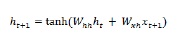
Next, we can repeat the process of updating the hidden state for the third and final step in the sequence as below −

And when we have processed all the above steps in the sequence, we can calculate the output as follows −

For the above formula, we have used a third set of weights and the hidden state from the final time step.
Advanced Recurrent Units
The main issue with basic recurrent layer is of vanishing gradient problem and due to this it is not very good at learning long-term correlations. In simple words basic recurrent layer does not handle long sequences very well. That’s the reason some other recurrent layer types that are much more suited for working with longer sequences are as follows −
Long-Short Term Memory (LSTM)

Long-short term memory (LSTMs) networks were introduced by Hochreiter & Schmidhuber. It solved the problem of getting a basic recurrent layer to remember things for a long time. The architecture of LSTM is given above in the diagram. As we can see it has input neurons, memory cells, and output neurons. In order to combat the vanishing gradient problem, Long-short term memory networks use an explicit memory cell (stores the previous values) and the following gates −
Forget gate− As name implies, it tells the memory cell to forget the previous values. The memory cell stores the values until the gate i.e. ‘forget gate’ tells it to forget them.
Input gate− As name implies, it adds new stuff to the cell.
Output gate− As name implies, output gate decides when to pass along the vectors from the cell to the next hidden state.
Gated Recurrent Units (GRUs)

Gradient recurrent units (GRUs) is a slight variation of LSTMs network. It has one less gate and are wired slightly different than LSTMs. Its architecture is shown in the above diagram. It has input neurons, gated memory cells, and output neurons. Gated Recurrent Units network has the following two gates −
Update gate− It determines the following two things−
What amount of the information should be kept from the last state?
What amount of the information should be let in from the previous layer?
Reset gate− The functionality of reset gate is much like that of forget gate of LSTMs network. The only difference is that it is located slightly differently.
In contrast to Long-short term memory network, Gated Recurrent Unit networks are slightly faster and easier to run.
Creating RNN structure
Before we can start, making prediction about the output from any of our data source, we need to first construct RNN and constructing RNN is quite same as we had build regular neural network in previous section. Following is the code to build one−
from cntk.losses import squared_error
from cntk.io import CTFDeserializer, MinibatchSource, INFINITELY_REPEAT, StreamDefs, StreamDef
from cntk.learners import adam
from cntk.logging import ProgressPrinter
from cntk.train import TestConfig
BATCH_SIZE = 14 * 10
EPOCH_SIZE = 12434
EPOCHS = 10
Staking multiple layers
We can also stack multiple recurrent layers in CNTK. For example, we can use the following combination of layers−
from cntk import sequence, default_options, input_variable
from cntk.layers import Recurrence, LSTM, Dropout, Dense, Sequential, Fold
features = sequence.input_variable(1)
with default_options(initial_state = 0.1):
   model = Sequential([
      Fold(LSTM(15)),
      Dense(1)
   ])(features)
target = input_variable(1, dynamic_axes=model.dynamic_axes)
As we can see in the above code, we have the following two ways in which we can model RNN in CNTK −
First, if we only want the final output of a recurrent layer, we can use the Fold layer in combination with a recurrent layer, such as GRU, LSTM, or even RNNStep.
Second, as an alternative way, we can also use the Recurrence block.
Training RNN with time series data
Once we build the model, let’s see how we can train RNN in CNTK −
from cntk import Function
@Function
def criterion_factory(z, t):
   loss = squared_error(z, t)
   metric = squared_error(z, t)
   return loss, metric
loss = criterion_factory(model, target)
learner = adam(model.parameters, lr=0.005, momentum=0.9)
Now to load the data into the training process, we must have to deserialize sequences from a set of CTF files. Following code have the create_datasource function, which is a useful utility function to create both the training and test datasource.
target_stream = StreamDef(field='target', shape=1, is_sparse=False)
features_stream = StreamDef(field='features', shape=1, is_sparse=False)
deserializer = CTFDeserializer(filename, StreamDefs(features=features_stream, target=target_stream))
   datasource = MinibatchSource(deserializer, randomize=True, max_sweeps=sweeps)
return datasource
train_datasource = create_datasource('Training data filename.ctf')#we need to provide the location of training file we created from our dataset.
test_datasource = create_datasource('Test filename.ctf', sweeps=1) #we need to provide the location of testing file we created from our dataset.
Now, as we have setup the data sources, model and the loss function, we can start the training process. It is quite similar as we did in previous sections with basic neural networks.
progress_writer = ProgressPrinter(0)
test_config = TestConfig(test_datasource)
input_map = {
   features: train_datasource.streams.features,
   target: train_datasource.streams.target
}
history = loss.train(
   train_datasource,
   epoch_size=EPOCH_SIZE,
   parameter_learners=[learner],
   model_inputs_to_streams=input_map,
   callbacks=[progress_writer, test_config],
   minibatch_size=BATCH_SIZE,
   max_epochs=EPOCHS
)
We will get the output similar as follows −
Output−
average  since  average  since  examples
loss      last  metric  last
------------------------------------------------------
Learning rate per minibatch: 0.005
0.4      0.4    0.4      0.4      19
0.4      0.4    0.4      0.4      59
0.452    0.495  0.452    0.495   129
[…]
Validating the model
Actually redicting with a RNN is quite similar to making predictions with any other CNK model. The only difference is that, we need to provide sequences rather than single samples.
Now, as our RNN is finally done with training, we can validate the model by testing it using a few samples sequence as follows −
import pickle
with open('test_samples.pkl', 'rb') as test_file:
test_samples = pickle.load(test_file)
model(test_samples) * NORMALIZE
Output−
array([[ 8081.7905],
[16597.693 ],
[13335.17 ],
...,
[11275.804 ],
[15621.697 ],
[16875.555 ]], dtype=float32)