Pythonパンダ-クイックガイド
Pandasは、強力なデータ構造を使用した高性能のデータ操作および分析ツールを提供するオープンソースのPythonライブラリです。パンダという名前は、パネルデータ(多次元データからの計量経済学)という言葉に由来しています。
2008年、開発者のWes McKinneyは、データ分析用の高性能で柔軟なツールが必要なときにパンダの開発を開始しました。
Pandasの前は、Pythonは主にデータの変更と準備に使用されていました。データ分析への貢献はほとんどありませんでした。パンダはこの問題を解決しました。Pandasを使用すると、データの出所に関係なく、データの処理と分析において、ロード、準備、操作、モデル化、分析の5つの典型的なステップを実行できます。
Python with Pandasは、金融、経済、統計、分析などの学術および商業分野を含む幅広い分野で使用されています。
パンダの主な機能
- デフォルトのカスタマイズされたインデックスを使用した、高速で効率的なDataFrameオブジェクト。
- さまざまなファイル形式からインメモリデータオブジェクトにデータをロードするためのツール。
- データの調整と欠落データの統合処理。
- 日付セットの再形成とピボット。
- 大規模なデータセットのラベルベースのスライス、インデックス作成、サブセット化。
- データ構造の列は削除または挿入できます。
- 集計と変換のためにデータでグループ化します。
- データの高性能なマージと結合。
- 時系列機能。
標準のPythonディストリビューションは、Pandasモジュールにバンドルされていません。軽量の代替手段は、人気のあるPythonパッケージインストーラーを使用してNumPyをインストールすることです。pip.
pip install pandasAnaconda Pythonパッケージをインストールすると、Pandasはデフォルトで次のようにインストールされます-
ウィンドウズ
Anaconda (から https://www.continuum.io)はSciPyスタック用の無料のPythonディストリビューションです。LinuxとMacでも利用できます。
Canopy ((https://www.enthought.com/products/canopy/)は、Windows、Linux、およびMac用の完全なSciPyスタックを備えた無料および商用の配布として利用できます。
Python(x、y)は、WindowsOS用のSciPyスタックとSpyderIDEを備えた無料のPythonディストリビューションです。(からダウンロード可能http://python-xy.github.io/)
Linux
それぞれのLinuxディストリビューションのパッケージマネージャーは、SciPyスタックに1つ以上のパッケージをインストールするために使用されます。
For Ubuntu Users
sudo apt-get install python-numpy python-scipy python-matplotlibipythonipythonnotebook
python-pandas python-sympy python-nose
For Fedora Users
sudo yum install numpyscipy python-matplotlibipython python-pandas sympy
python-nose atlas-devel
パンダは次の3つのデータ構造を扱います-
- Series
- DataFrame
- Panel
これらのデータ構造は、Numpy配列の上に構築されているため、高速です。
寸法と説明
これらのデータ構造を考える最良の方法は、高次元のデータ構造が低次元のデータ構造のコンテナーであるということです。たとえば、DataFrameはSeriesのコンテナであり、PanelはDataFrameのコンテナです。
| データ構造 | 寸法 | 説明 |
|---|---|---|
| シリーズ | 1 | サイズ不変の1Dラベル付き同種配列。 |
| データフレーム | 2 | 不均一に型付けされる可能性のある列を持つ、一般的な2Dラベル付きのサイズ変更可能な表形式の構造。 |
| パネル | 3 | 一般的な3Dラベル付き、サイズ変更可能な配列。 |
2次元以上の配列を作成して処理するのは面倒な作業であり、関数を作成するときにデータセットの方向を考慮する必要があります。しかし、パンダのデータ構造を使用すると、ユーザーの精神的な労力が軽減されます。
たとえば、表形式のデータ(DataFrame)の場合、意味的には index (行)と columns 軸0と軸1ではなく。
可変性
すべてのパンダのデータ構造は値が変更可能(変更可能)であり、シリーズを除いてすべてサイズが変更可能です。シリーズはサイズ不変です。
Note− DataFrameは広く使用されており、最も重要なデータ構造の1つです。パネルの使用量ははるかに少なくなります。
シリーズ
シリーズは、同種のデータを持つ構造のような1次元配列です。たとえば、次のシリーズは整数10、23、56、…のコレクションです。
| 10 | 23 | 56 | 17 | 52 | 61 | 73 | 90 | 26 | 72 |
キーポイント
- 均質なデータ
- サイズ不変
- 可変データの値
DataFrame
DataFrameは、異種データを含む2次元配列です。例えば、
| 名前 | 年齢 | 性別 | 評価 |
|---|---|---|---|
| スティーブ | 32 | 男性 | 3.45 |
| リア | 28 | 女性 | 4.6 |
| ヴィン | 45 | 男性 | 3.9 |
| ケイティ | 38 | 女性 | 2.78 |
この表は、組織の営業チームのデータと全体的なパフォーマンス評価を表しています。データは行と列で表されます。各列は属性を表し、各行は人を表します。
列のデータ型
4列のデータ型は次のとおりです。
| カラム | タイプ |
|---|---|
| 名前 | ストリング |
| 年齢 | 整数 |
| 性別 | ストリング |
| 評価 | 浮く |
キーポイント
- 異種データ
- サイズ可変
- データ可変
パネル
Panelは、異種データを含む3次元データ構造です。パネルをグラフィック表現で表現するのは困難です。ただし、パネルはDataFrameのコンテナとして説明できます。
キーポイント
- 異種データ
- サイズ可変
- データ可変
Seriesは、任意のタイプ(整数、文字列、浮動小数点数、Pythonオブジェクトなど)のデータを保持できる1次元のラベル付き配列です。軸ラベルはまとめてインデックスと呼ばれます。
pandas.Series
パンダシリーズは、次のコンストラクターを使用して作成できます-
pandas.Series( data, index, dtype, copy)コンストラクターのパラメーターは次のとおりです-
| シニア番号 | パラメータと説明 |
|---|---|
| 1 | data データは、ndarray、list、constantsなどのさまざまな形式を取ります |
| 2 | index インデックス値は、データと同じ長さで、一意でハッシュ可能である必要があります。デフォルトnp.arange(n) インデックスが渡されない場合。 |
| 3 | dtype dtypeはデータ型用です。Noneの場合、データ型が推測されます |
| 4 | copy データをコピーします。デフォルトFalse |
シリーズは、次のようなさまざまな入力を使用して作成できます。
- Array
- Dict
- スカラー値または定数
空のシリーズを作成する
作成できる基本シリーズは空シリーズです。
例
#import the pandas library and aliasing as pd
import pandas as pd
s = pd.Series()
print s
その output 次のとおりです-
Series([], dtype: float64)ndarrayからシリーズを作成する
データがndarrayの場合、渡されるインデックスは同じ長さである必要があります。インデックスが渡されない場合、デフォルトでインデックスはrange(n) どこ n は配列の長さ、つまり[0,1,2,3…。 range(len(array))-1].
例1
#import the pandas library and aliasing as pd
import pandas as pd
import numpy as np
data = np.array(['a','b','c','d'])
s = pd.Series(data)
print s
その output 次のとおりです-
0   a
1   b
2   c
3   d
dtype: object
インデックスを渡さなかったため、デフォルトでは、0から0までの範囲のインデックスが割り当てられました。 len(data)-1、つまり、0から3。
例2
#import the pandas library and aliasing as pd
import pandas as pd
import numpy as np
data = np.array(['a','b','c','d'])
s = pd.Series(data,index=[100,101,102,103])
print s
その output 次のとおりです-
100  a
101  b
102  c
103  d
dtype: object
ここにインデックス値を渡しました。これで、カスタマイズされたインデックス値が出力に表示されます。
dictからシリーズを作成する
A dict入力として渡すことができ、インデックスが指定されていない場合、辞書キーはソートされた順序で取得されてインデックスが作成されます。場合index が渡されると、インデックスのラベルに対応するデータの値が引き出されます。
例1
#import the pandas library and aliasing as pd
import pandas as pd
import numpy as np
data = {'a' : 0., 'b' : 1., 'c' : 2.}
s = pd.Series(data)
print s
その output 次のとおりです-
a 0.0
b 1.0
c 2.0
dtype: float64
Observe −辞書キーはインデックスの作成に使用されます。
例2
#import the pandas library and aliasing as pd
import pandas as pd
import numpy as np
data = {'a' : 0., 'b' : 1., 'c' : 2.}
s = pd.Series(data,index=['b','c','d','a'])
print s
その output 次のとおりです-
b 1.0
c 2.0
d NaN
a 0.0
dtype: float64
Observe −インデックスの順序は保持され、欠落している要素はNaN(数値ではない)で埋められます。
スカラーからシリーズを作成する
データがスカラー値の場合、インデックスを指定する必要があります。値は、の長さに一致するように繰り返されますindex
#import the pandas library and aliasing as pd
import pandas as pd
import numpy as np
s = pd.Series(5, index=[0, 1, 2, 3])
print s
その output 次のとおりです-
0  5
1  5
2  5
3  5
dtype: int64
位置のあるシリーズからのデータへのアクセス
シリーズのデータは、のデータと同様にアクセスできます。 ndarray.
例1
最初の要素を取得します。すでに知っているように、カウントは配列のゼロから始まります。つまり、最初の要素はゼロ番目の位置に格納されます。
import pandas as pd
s = pd.Series([1,2,3,4,5],index = ['a','b','c','d','e'])

#retrieve the first element
print s[0]
その output 次のとおりです-
1例2
シリーズの最初の3つの要素を取得します。その前に:を挿入すると、そのインデックス以降のすべてのアイテムが抽出されます。2つのパラメーター(それらの間に:を含む)が使用されている場合、2つのインデックス間のアイテム(停止インデックスを含まない)
import pandas as pd
s = pd.Series([1,2,3,4,5],index = ['a','b','c','d','e'])

#retrieve the first three element
print s[:3]
その output 次のとおりです-
a  1
b  2
c  3
dtype: int64
例3
最後の3つの要素を取得します。
import pandas as pd
s = pd.Series([1,2,3,4,5],index = ['a','b','c','d','e'])

#retrieve the last three element
print s[-3:]
その output 次のとおりです-
c  3
d  4
e  5
dtype: int64
ラベル(インデックス)を使用してデータを取得する
シリーズは固定サイズのようなものです dict インデックスラベルで値を取得および設定できるという点で。
例1
インデックスラベル値を使用して単一の要素を取得します。
import pandas as pd
s = pd.Series([1,2,3,4,5],index = ['a','b','c','d','e'])

#retrieve a single element
print s['a']
その output 次のとおりです-
1例2
インデックスラベル値のリストを使用して複数の要素を取得します。
import pandas as pd
s = pd.Series([1,2,3,4,5],index = ['a','b','c','d','e'])

#retrieve multiple elements
print s[['a','c','d']]
その output 次のとおりです-
a  1
c  3
d  4
dtype: int64
例3
ラベルが含まれていない場合、例外が発生します。
import pandas as pd
s = pd.Series([1,2,3,4,5],index = ['a','b','c','d','e'])

#retrieve multiple elements
print s['f']
その output 次のとおりです-
…
KeyError: 'f'
データフレームは2次元のデータ構造です。つまり、データは行と列に表形式で配置されます。
DataFrameの機能
- 潜在的に列は異なるタイプです
- サイズ–変更可能
- ラベル付きの軸(行と列)
- 行と列に対して算術演算を実行できます
構造
学生のデータを使用してデータフレームを作成していると仮定します。

これは、SQLテーブルまたはスプレッドシートのデータ表現と考えることができます。
pandas.DataFrame
pandas DataFrameは、次のコンストラクターを使用して作成できます-
pandas.DataFrame( data, index, columns, dtype, copy)コンストラクターのパラメーターは次のとおりです-
| シニア番号 | パラメータと説明 |
|---|---|
| 1 | data データは、ndarray、series、map、lists、dict、constants、および別のDataFrameなどのさまざまな形式を取ります。 |
| 2 | index 行ラベルの場合、結果のフレームに使用されるインデックスは、インデックスが渡されない場合、オプションのデフォルトnp.arange(n)です。 |
| 3 | columns 列ラベルの場合、オプションのデフォルト構文は--np.arange(n)です。これは、インデックスが渡されない場合にのみ当てはまります。 |
| 4 | dtype 各列のデータ型。 |
| 5 | copy デフォルトがFalseの場合、このコマンド(またはそれが何であれ)はデータのコピーに使用されます。 |
DataFrameを作成する
pandas DataFrameは、次のようなさまざまな入力を使用して作成できます。
- Lists
- dict
- Series
- ゴツゴツしたndarrays
- 別のDataFrame
この章の後続のセクションでは、これらの入力を使用してDataFrameを作成する方法を説明します。
空のデータフレームを作成する
作成できる基本的なDataFrameはEmptyDataframeです。
例
#import the pandas library and aliasing as pd
import pandas as pd
df = pd.DataFrame()
print df
その output 次のとおりです-
Empty DataFrame
Columns: []
Index: []
リストからDataFrameを作成する
DataFrameは、単一のリストまたはリストのリストを使用して作成できます。
例1
import pandas as pd
data = [1,2,3,4,5]
df = pd.DataFrame(data)
print df
その output 次のとおりです-
0
0    1
1    2
2    3
3    4
4    5
例2
import pandas as pd
data = [['Alex',10],['Bob',12],['Clarke',13]]
df = pd.DataFrame(data,columns=['Name','Age'])
print df
その output 次のとおりです-
Name      Age
0     Alex      10
1     Bob       12
2     Clarke    13
例3
import pandas as pd
data = [['Alex',10],['Bob',12],['Clarke',13]]
df = pd.DataFrame(data,columns=['Name','Age'],dtype=float)
print df
その output 次のとおりです-
Name     Age
0     Alex     10.0
1     Bob      12.0
2     Clarke   13.0
Note −観察してください dtype パラメータは、Age列のタイプを浮動小数点に変更します。
ndarrays / ListsのディクトからDataFrameを作成します
全ての ndarrays同じ長さである必要があります。インデックスが渡される場合、インデックスの長さは配列の長さと等しくなければなりません。
インデックスが渡されない場合、デフォルトでは、インデックスはrange(n)になります。ここで、 n は配列の長さです。
例1
import pandas as pd
data = {'Name':['Tom', 'Jack', 'Steve', 'Ricky'],'Age':[28,34,29,42]}
df = pd.DataFrame(data)
print df
その output 次のとおりです-
Age      Name
0     28        Tom
1     34       Jack
2     29      Steve
3 42 RickyNote−値0、1、2、3を観察します。これらは、関数range(n)を使用してそれぞれに割り当てられるデフォルトのインデックスです。
例2
次に、配列を使用してインデックス付きのDataFrameを作成しましょう。
import pandas as pd
data = {'Name':['Tom', 'Jack', 'Steve', 'Ricky'],'Age':[28,34,29,42]}
df = pd.DataFrame(data, index=['rank1','rank2','rank3','rank4'])
print df
その output 次のとおりです-
Age    Name
rank1    28      Tom
rank2    34     Jack
rank3    29    Steve
rank4    42    Ricky
Note −観察してください index パラメータは、各行にインデックスを割り当てます。
ディクトのリストからDataFrameを作成する
辞書のリストを入力データとして渡して、DataFrameを作成できます。辞書キーは、デフォルトで列名として使用されます。
例1
次の例は、辞書のリストを渡してDataFrameを作成する方法を示しています。
import pandas as pd
data = [{'a': 1, 'b': 2},{'a': 5, 'b': 10, 'c': 20}]
df = pd.DataFrame(data)
print df
その output 次のとおりです-
a    b      c
0   1   2     NaN
1   5   10   20.0
Note −観察してください、NaN(数字ではありません)が欠落している領域に追加されています。
例2
次の例は、辞書のリストと行インデックスを渡してDataFrameを作成する方法を示しています。
import pandas as pd
data = [{'a': 1, 'b': 2},{'a': 5, 'b': 10, 'c': 20}]
df = pd.DataFrame(data, index=['first', 'second'])
print df
その output 次のとおりです-
a   b       c
first   1   2     NaN
second  5   10   20.0
例3
次の例は、辞書、行インデックス、および列インデックスのリストを使用してDataFrameを作成する方法を示しています。
import pandas as pd
data = [{'a': 1, 'b': 2},{'a': 5, 'b': 10, 'c': 20}]

#With two column indices, values same as dictionary keys
df1 = pd.DataFrame(data, index=['first', 'second'], columns=['a', 'b'])

#With two column indices with one index with other name
df2 = pd.DataFrame(data, index=['first', 'second'], columns=['a', 'b1'])
print df1
print df2
その output 次のとおりです-
#df1 output
         a  b
first    1  2
second   5  10

#df2 output
         a  b1
first    1  NaN
second 5 NaNNote−注意してください。df2DataFrameは、辞書キー以外の列インデックスで作成されます。したがって、NaNを所定の位置に追加しました。一方、df1は辞書キーと同じ列インデックスで作成されるため、NaNが追加されます。
Dict ofSeriesからDataFrameを作成する
シリーズのディクショナリを渡して、DataFrameを形成できます。結果のインデックスは、渡されたすべてのシリーズインデックスの和集合です。
例
import pandas as pd

d = {'one' : pd.Series([1, 2, 3], index=['a', 'b', 'c']),
   'two' : pd.Series([1, 2, 3, 4], index=['a', 'b', 'c', 'd'])}

df = pd.DataFrame(d)
print df
その output 次のとおりです-
one    two
a     1.0    1
b     2.0    2
c     3.0    3
d     NaN    4
Note −シリーズ1の場合、ラベルがないことに注意してください ‘d’ 合格しましたが、結果として、 d ラベル、NaNにはNaNが追加されます。
今理解しましょう column selection, addition、および deletion 例を通して。
列の選択
これは、DataFrameから列を選択することで理解できます。
例
import pandas as pd

d = {'one' : pd.Series([1, 2, 3], index=['a', 'b', 'c']),
   'two' : pd.Series([1, 2, 3, 4], index=['a', 'b', 'c', 'd'])}

df = pd.DataFrame(d)
print df ['one']
その output 次のとおりです-
a     1.0
b     2.0
c     3.0
d     NaN
Name: one, dtype: float64
列の追加
これは、既存のデータフレームに新しい列を追加することで理解できます。
例
import pandas as pd

d = {'one' : pd.Series([1, 2, 3], index=['a', 'b', 'c']),
   'two' : pd.Series([1, 2, 3, 4], index=['a', 'b', 'c', 'd'])}

df = pd.DataFrame(d)

# Adding a new column to an existing DataFrame object with column label by passing new series

print ("Adding a new column by passing as Series:")
df['three']=pd.Series([10,20,30],index=['a','b','c'])
print df

print ("Adding a new column using the existing columns in DataFrame:")
df['four']=df['one']+df['three']

print df
その output 次のとおりです-
Adding a new column by passing as Series:
     one   two   three
a    1.0    1    10.0
b    2.0    2    20.0
c    3.0    3    30.0
d    NaN    4    NaN

Adding a new column using the existing columns in DataFrame:
      one   two   three    four
a     1.0    1    10.0     11.0
b     2.0    2    20.0     22.0
c     3.0    3    30.0     33.0
d     NaN    4     NaN     NaN
列の削除
列は削除またはポップできます。例を挙げて、その方法を理解しましょう。
例
# Using the previous DataFrame, we will delete a column
# using del function
import pandas as pd

d = {'one' : pd.Series([1, 2, 3], index=['a', 'b', 'c']),
   'two' : pd.Series([1, 2, 3, 4], index=['a', 'b', 'c', 'd']),
   'three' : pd.Series([10,20,30], index=['a','b','c'])}

df = pd.DataFrame(d)
print ("Our dataframe is:")
print df

# using del function
print ("Deleting the first column using DEL function:")
del df['one']
print df

# using pop function
print ("Deleting another column using POP function:")
df.pop('two')
print df
その output 次のとおりです-
Our dataframe is:
      one   three  two
a     1.0    10.0   1
b     2.0    20.0   2
c     3.0    30.0   3
d     NaN     NaN   4

Deleting the first column using DEL function:
      three    two
a     10.0     1
b     20.0     2
c     30.0     3
d     NaN      4

Deleting another column using POP function:
   three
a  10.0
b  20.0
c  30.0
d  NaN
行の選択、追加、および削除
例を通して、行の選択、追加、削除について理解します。選択の概念から始めましょう。
ラベルによる選択
行ラベルをに渡すことで行を選択できます loc 関数。
import pandas as pd

d = {'one' : pd.Series([1, 2, 3], index=['a', 'b', 'c']),
   'two' : pd.Series([1, 2, 3, 4], index=['a', 'b', 'c', 'd'])}

df = pd.DataFrame(d)
print df.loc['b']
その output 次のとおりです-
one 2.0
two 2.0
Name: b, dtype: float64
結果は、DataFrameの列名としてラベルを持つシリーズです。また、シリーズの名前は、シリーズを取得するためのラベルです。
整数位置による選択
行は整数の位置をに渡すことで選択できます iloc 関数。
import pandas as pd

d = {'one' : pd.Series([1, 2, 3], index=['a', 'b', 'c']),
   'two' : pd.Series([1, 2, 3, 4], index=['a', 'b', 'c', 'd'])}

df = pd.DataFrame(d)
print df.iloc[2]
その output 次のとおりです-
one   3.0
two   3.0
Name: c, dtype: float64
スライス行
':'演算子を使用して複数の行を選択できます。
import pandas as pd

d = {'one' : pd.Series([1, 2, 3], index=['a', 'b', 'c']),
   'two' : pd.Series([1, 2, 3, 4], index=['a', 'b', 'c', 'd'])}

df = pd.DataFrame(d)
print df[2:4]
その output 次のとおりです-
one  two
c  3.0    3
d  NaN    4
行の追加
を使用してDataFrameに新しい行を追加します append関数。この関数は、最後に行を追加します。
import pandas as pd

df = pd.DataFrame([[1, 2], [3, 4]], columns = ['a','b'])
df2 = pd.DataFrame([[5, 6], [7, 8]], columns = ['a','b'])

df = df.append(df2)
print df
その output 次のとおりです-
a  b
0  1  2
1  3  4
0  5  6
1  7  8
行の削除
インデックスラベルを使用して、DataFrameから行を削除または削除します。ラベルが重複している場合、複数の行が削除されます。
観察すると、上記の例では、ラベルが重複しています。ラベルを削除して、削除される行数を確認しましょう。
import pandas as pd

df = pd.DataFrame([[1, 2], [3, 4]], columns = ['a','b'])
df2 = pd.DataFrame([[5, 6], [7, 8]], columns = ['a','b'])

df = df.append(df2)

# Drop rows with label 0
df = df.drop(0)

print df
その output 次のとおりです-
a b
1 3 4
1 7 8
上記の例では、2つの行に同じラベル0が含まれているため、2つの行が削除されました。
A panelデータの3Dコンテナです。用語Panel data 計量経済学から派生し、パンダの名前に部分的に責任があります- pan(el)-da(ta)-s。
3つの軸の名前は、パネルデータを含む操作を説明するための意味的な意味を与えることを目的としています。彼らは-
items −軸0、各項目は内部に含まれるDataFrameに対応します。
major_axis −軸1は、各DataFrameのインデックス(行)です。
minor_axis −軸2は、各DataFrameの列です。
pandas.Panel()
パネルは、次のコンストラクターを使用して作成できます-
pandas.Panel(data, items, major_axis, minor_axis, dtype, copy)コンストラクターのパラメーターは次のとおりです-
| パラメータ | 説明 |
|---|---|
| データ | データは、ndarray、series、map、lists、dict、constants、および別のDataFrameなどのさまざまな形式を取ります |
| アイテム | axis = 0 |
| major_axis | axis = 1 |
| minor_axis | axis = 2 |
| dtype | 各列のデータ型 |
| コピー | データをコピーします。デフォルト、false |
パネルの作成
パネルは、次のような複数の方法を使用して作成できます。
- ndarraysから
- DataFramesのdictから
3Dndarrayから
# creating an empty panel
import pandas as pd
import numpy as np

data = np.random.rand(2,4,5)
p = pd.Panel(data)
print p
その output 次のとおりです-
<class 'pandas.core.panel.Panel'>
Dimensions: 2 (items) x 4 (major_axis) x 5 (minor_axis)
Items axis: 0 to 1
Major_axis axis: 0 to 3
Minor_axis axis: 0 to 4
Note −空のパネルと上のパネルの寸法を観察します。すべてのオブジェクトが異なります。
DataFrameオブジェクトのdictから
#creating an empty panel
import pandas as pd
import numpy as np

data = {'Item1' : pd.DataFrame(np.random.randn(4, 3)),
   'Item2' : pd.DataFrame(np.random.randn(4, 2))}
p = pd.Panel(data)
print p
その output 次のとおりです-
Dimensions: 2 (items) x 4 (major_axis) x 3 (minor_axis)
Items axis: Item1 to Item2
Major_axis axis: 0 to 3
Minor_axis axis: 0 to 2
空のパネルを作成する
空のパネルは、次のようにPanelコンストラクターを使用して作成できます。
#creating an empty panel
import pandas as pd
p = pd.Panel()
print p
その output 次のとおりです-
<class 'pandas.core.panel.Panel'>
Dimensions: 0 (items) x 0 (major_axis) x 0 (minor_axis)
Items axis: None
Major_axis axis: None
Minor_axis axis: None
パネルからのデータの選択
−を使用してパネルからデータを選択します
- Items
- Major_axis
- Minor_axis
アイテムの使用
# creating an empty panel
import pandas as pd
import numpy as np
data = {'Item1' : pd.DataFrame(np.random.randn(4, 3)),
   'Item2' : pd.DataFrame(np.random.randn(4, 2))}
p = pd.Panel(data)
print p['Item1']
その output 次のとおりです-
0          1          2
0    0.488224  -0.128637   0.930817
1    0.417497   0.896681   0.576657
2   -2.775266   0.571668   0.290082
3 -0.400538 -0.144234 1.1105352つのアイテムがあり、item1を取得しました。結果は、4行3列のDataFrameです。Major_axis そして Minor_axis 寸法。
major_axisの使用
この方法を使用してデータにアクセスできます panel.major_axis(index)。
# creating an empty panel
import pandas as pd
import numpy as np
data = {'Item1' : pd.DataFrame(np.random.randn(4, 3)),
   'Item2' : pd.DataFrame(np.random.randn(4, 2))}
p = pd.Panel(data)
print p.major_xs(1)
その output 次のとおりです-
Item1       Item2
0   0.417497    0.748412
1   0.896681   -0.557322
2   0.576657       NaN
minor_axisの使用
この方法を使用してデータにアクセスできます panel.minor_axis(index).
# creating an empty panel
import pandas as pd
import numpy as np
data = {'Item1' : pd.DataFrame(np.random.randn(4, 3)),
   'Item2' : pd.DataFrame(np.random.randn(4, 2))}
p = pd.Panel(data)
print p.minor_xs(1)
その output 次のとおりです-
Item1       Item2
0   -0.128637   -1.047032
1    0.896681   -0.557322
2    0.571668    0.431953
3   -0.144234    1.302466
Note −寸法の変化を観察します。
ここまでで、3つのPandasDataStructuresとそれらの作成方法について学習しました。リアルタイムデータ処理における重要性のため、主にDataFrameオブジェクトに焦点を当て、他のいくつかのDataStructureについても説明します。
シリーズの基本機能
| シニア番号 | 属性またはメソッドと説明 |
|---|---|
| 1 | axes 行軸ラベルのリストを返します |
| 2 | dtype オブジェクトのdtypeを返します。 |
| 3 | empty シリーズが空の場合はTrueを返します。 |
| 4 | ndim 定義1により、基になるデータの次元数を返します。 |
| 5 | size 基になるデータの要素の数を返します。 |
| 6 | values シリーズをndarrayとして返します。 |
| 7 | head() 最初のn行を返します。 |
| 8 | tail() 最後のn行を返します。 |
シリーズを作成して、上記のすべての表形式の属性操作を見てみましょう。
例
import pandas as pd
import numpy as np

#Create a series with 100 random numbers
s = pd.Series(np.random.randn(4))
print s
その output 次のとおりです-
0   0.967853
1  -0.148368
2  -1.395906
3  -1.758394
dtype: float64
軸
シリーズのラベルのリストを返します。
import pandas as pd
import numpy as np

#Create a series with 100 random numbers
s = pd.Series(np.random.randn(4))
print ("The axes are:")
print s.axes
その output 次のとおりです-
The axes are:
[RangeIndex(start=0, stop=4, step=1)]
上記の結果は、0から5までの値のリストのコンパクトな形式、つまり[0,1,2,3,4]です。
空の
オブジェクトが空かどうかを示すブール値を返します。Trueは、オブジェクトが空であることを示します。
import pandas as pd
import numpy as np

#Create a series with 100 random numbers
s = pd.Series(np.random.randn(4))
print ("Is the Object empty?")
print s.empty
その output 次のとおりです-
Is the Object empty?
False
ndim
オブジェクトの次元数を返します。定義上、シリーズは1Dデータ構造であるため、
import pandas as pd
import numpy as np

#Create a series with 4 random numbers
s = pd.Series(np.random.randn(4))
print s

print ("The dimensions of the object:")
print s.ndim
その output 次のとおりです-
0   0.175898
1   0.166197
2  -0.609712
3  -1.377000
dtype: float64

The dimensions of the object:
1
サイズ
シリーズのサイズ(長さ)を返します。
import pandas as pd
import numpy as np

#Create a series with 4 random numbers
s = pd.Series(np.random.randn(2))
print s
print ("The size of the object:")
print s.size
その output 次のとおりです-
0   3.078058
1  -1.207803
dtype: float64

The size of the object:
2
値
系列の実際のデータを配列として返します。
import pandas as pd
import numpy as np

#Create a series with 4 random numbers
s = pd.Series(np.random.randn(4))
print s

print ("The actual data series is:")
print s.values
その output 次のとおりです-
0   1.787373
1  -0.605159
2   0.180477
3  -0.140922
dtype: float64

The actual data series is:
[ 1.78737302 -0.60515881 0.18047664 -0.1409218 ]
ヘッド&テール
SeriesまたはDataFrameオブジェクトの小さなサンプルを表示するには、head()メソッドとtail()メソッドを使用します。
head() 最初を返します n行(インデックス値を確認してください)。表示する要素のデフォルト数は5ですが、カスタム数を渡すこともできます。
import pandas as pd
import numpy as np

#Create a series with 4 random numbers
s = pd.Series(np.random.randn(4))
print ("The original series is:")
print s

print ("The first two rows of the data series:")
print s.head(2)
その output 次のとおりです-
The original series is:
0   0.720876
1  -0.765898
2   0.479221
3  -0.139547
dtype: float64

The first two rows of the data series:
0   0.720876
1  -0.765898
dtype: float64
tail() 最後を返します n行(インデックス値を確認してください)。表示する要素のデフォルト数は5ですが、カスタム数を渡すこともできます。
import pandas as pd
import numpy as np

#Create a series with 4 random numbers
s = pd.Series(np.random.randn(4))
print ("The original series is:")
print s

print ("The last two rows of the data series:")
print s.tail(2)
その output 次のとおりです-
The original series is:
0 -0.655091
1 -0.881407
2 -0.608592
3 -2.341413
dtype: float64

The last two rows of the data series:
2 -0.608592
3 -2.341413
dtype: float64
DataFrameの基本機能
ここで、DataFrameの基本機能とは何かを理解しましょう。次の表に、DataFrameの基本機能に役立つ重要な属性またはメソッドを示します。
| シニア番号 | 属性またはメソッドと説明 |
|---|---|
| 1 | T 行と列を転置します。 |
| 2 | axes 行軸ラベルと列軸ラベルのみをメンバーとするリストを返します。 |
| 3 | dtypes このオブジェクトのdtypeを返します。 |
| 4 | empty NDFrameが完全に空の場合はTrue [アイテムなし]。軸のいずれかが長さ0の場合。 |
| 5 | ndim 軸の数/配列の次元。 |
| 6 | shape DataFrameの次元を表すタプルを返します。 |
| 7 | size NDFrame内の要素の数。 |
| 8 | values NDFrameのNumpy表現。 |
| 9 | head() 最初のn行を返します。 |
| 10 | tail() 最後のn行を返します。 |
DataFrameを作成して、上記の属性がどのように機能するかを見てみましょう。
例
import pandas as pd
import numpy as np

#Create a Dictionary of series
d = {'Name':pd.Series(['Tom','James','Ricky','Vin','Steve','Smith','Jack']),
   'Age':pd.Series([25,26,25,23,30,29,23]),
   'Rating':pd.Series([4.23,3.24,3.98,2.56,3.20,4.6,3.8])}

#Create a DataFrame
df = pd.DataFrame(d)
print ("Our data series is:")
print df
その output 次のとおりです-
Our data series is:
    Age   Name    Rating
0   25    Tom     4.23
1   26    James   3.24
2   25    Ricky   3.98
3   23    Vin     2.56
4   30    Steve   3.20
5   29    Smith   4.60
6   23    Jack    3.80
T(転置)
DataFrameの転置を返します。行と列が入れ替わります。
import pandas as pd
import numpy as np

# Create a Dictionary of series
d = {'Name':pd.Series(['Tom','James','Ricky','Vin','Steve','Smith','Jack']),
   'Age':pd.Series([25,26,25,23,30,29,23]),
   'Rating':pd.Series([4.23,3.24,3.98,2.56,3.20,4.6,3.8])}

# Create a DataFrame
df = pd.DataFrame(d)
print ("The transpose of the data series is:")
print df.T
その output 次のとおりです-
The transpose of the data series is:
         0     1       2      3      4      5       6
Age      25    26      25     23     30     29      23
Name     Tom   James   Ricky  Vin    Steve  Smith   Jack
Rating   4.23  3.24    3.98   2.56   3.2    4.6     3.8
軸
行軸ラベルと列軸ラベルのリストを返します。
import pandas as pd
import numpy as np

#Create a Dictionary of series
d = {'Name':pd.Series(['Tom','James','Ricky','Vin','Steve','Smith','Jack']),
   'Age':pd.Series([25,26,25,23,30,29,23]),
   'Rating':pd.Series([4.23,3.24,3.98,2.56,3.20,4.6,3.8])}

#Create a DataFrame
df = pd.DataFrame(d)
print ("Row axis labels and column axis labels are:")
print df.axes
その output 次のとおりです-
Row axis labels and column axis labels are:

[RangeIndex(start=0, stop=7, step=1), Index([u'Age', u'Name', u'Rating'],
dtype='object')]
dtypes
各列のデータ型を返します。
import pandas as pd
import numpy as np

#Create a Dictionary of series
d = {'Name':pd.Series(['Tom','James','Ricky','Vin','Steve','Smith','Jack']),
   'Age':pd.Series([25,26,25,23,30,29,23]),
   'Rating':pd.Series([4.23,3.24,3.98,2.56,3.20,4.6,3.8])}

#Create a DataFrame
df = pd.DataFrame(d)
print ("The data types of each column are:")
print df.dtypes
その output 次のとおりです-
The data types of each column are:
Age     int64
Name    object
Rating  float64
dtype: object
空の
オブジェクトが空かどうかを示すブール値を返します。Trueは、オブジェクトが空であることを示します。
import pandas as pd
import numpy as np

#Create a Dictionary of series
d = {'Name':pd.Series(['Tom','James','Ricky','Vin','Steve','Smith','Jack']),
   'Age':pd.Series([25,26,25,23,30,29,23]),
   'Rating':pd.Series([4.23,3.24,3.98,2.56,3.20,4.6,3.8])}

#Create a DataFrame
df = pd.DataFrame(d)
print ("Is the object empty?")
print df.empty
その output 次のとおりです-
Is the object empty?
False
ndim
オブジェクトの次元数を返します。定義上、DataFrameは2Dオブジェクトです。
import pandas as pd
import numpy as np

#Create a Dictionary of series
d = {'Name':pd.Series(['Tom','James','Ricky','Vin','Steve','Smith','Jack']),
   'Age':pd.Series([25,26,25,23,30,29,23]),
   'Rating':pd.Series([4.23,3.24,3.98,2.56,3.20,4.6,3.8])}

#Create a DataFrame
df = pd.DataFrame(d)
print ("Our object is:")
print df
print ("The dimension of the object is:")
print df.ndim
その output 次のとおりです-
Our object is:
      Age    Name     Rating
0     25     Tom      4.23
1     26     James    3.24
2     25     Ricky    3.98
3     23     Vin      2.56
4     30     Steve    3.20
5     29     Smith    4.60
6     23     Jack     3.80

The dimension of the object is:
2
形状
DataFrameの次元を表すタプルを返します。タプル(a、b)、ここでaは行数を表し、b 列の数を表します。
import pandas as pd
import numpy as np

#Create a Dictionary of series
d = {'Name':pd.Series(['Tom','James','Ricky','Vin','Steve','Smith','Jack']),
   'Age':pd.Series([25,26,25,23,30,29,23]),
   'Rating':pd.Series([4.23,3.24,3.98,2.56,3.20,4.6,3.8])}

#Create a DataFrame
df = pd.DataFrame(d)
print ("Our object is:")
print df
print ("The shape of the object is:")
print df.shape
その output 次のとおりです-
Our object is:
   Age   Name    Rating
0  25    Tom     4.23
1  26    James   3.24
2  25    Ricky   3.98
3  23    Vin     2.56
4  30    Steve   3.20
5  29    Smith   4.60
6  23    Jack    3.80

The shape of the object is:
(7, 3)
サイズ
DataFrame内の要素の数を返します。
import pandas as pd
import numpy as np

#Create a Dictionary of series
d = {'Name':pd.Series(['Tom','James','Ricky','Vin','Steve','Smith','Jack']),
   'Age':pd.Series([25,26,25,23,30,29,23]),
   'Rating':pd.Series([4.23,3.24,3.98,2.56,3.20,4.6,3.8])}

#Create a DataFrame
df = pd.DataFrame(d)
print ("Our object is:")
print df
print ("The total number of elements in our object is:")
print df.size
その output 次のとおりです-
Our object is:
    Age   Name    Rating
0   25    Tom     4.23
1   26    James   3.24
2   25    Ricky   3.98
3   23    Vin     2.56
4   30    Steve   3.20
5   29    Smith   4.60
6   23    Jack    3.80

The total number of elements in our object is:
21
値
DataFrame内の実際のデータをとして返します NDarray.
import pandas as pd
import numpy as np

#Create a Dictionary of series
d = {'Name':pd.Series(['Tom','James','Ricky','Vin','Steve','Smith','Jack']),
   'Age':pd.Series([25,26,25,23,30,29,23]),
   'Rating':pd.Series([4.23,3.24,3.98,2.56,3.20,4.6,3.8])}

#Create a DataFrame
df = pd.DataFrame(d)
print ("Our object is:")
print df
print ("The actual data in our data frame is:")
print df.values
その output 次のとおりです-
Our object is:
    Age   Name    Rating
0   25    Tom     4.23
1   26    James   3.24
2   25    Ricky   3.98
3   23    Vin     2.56
4   30    Steve   3.20
5   29    Smith   4.60
6   23    Jack    3.80
The actual data in our data frame is:
[[25 'Tom' 4.23]
[26 'James' 3.24]
[25 'Ricky' 3.98]
[23 'Vin' 2.56]
[30 'Steve' 3.2]
[29 'Smith' 4.6]
[23 'Jack' 3.8]]
ヘッド&テール
DataFrameオブジェクトの小さなサンプルを表示するには、 head() およびtail()メソッド。 head() 最初を返します n行(インデックス値を確認してください)。表示する要素のデフォルト数は5ですが、カスタム数を渡すこともできます。
import pandas as pd
import numpy as np

#Create a Dictionary of series
d = {'Name':pd.Series(['Tom','James','Ricky','Vin','Steve','Smith','Jack']),
   'Age':pd.Series([25,26,25,23,30,29,23]),
   'Rating':pd.Series([4.23,3.24,3.98,2.56,3.20,4.6,3.8])}

#Create a DataFrame
df = pd.DataFrame(d)
print ("Our data frame is:")
print df
print ("The first two rows of the data frame is:")
print df.head(2)
その output 次のとおりです-
Our data frame is:
    Age   Name    Rating
0   25    Tom     4.23
1   26    James   3.24
2   25    Ricky   3.98
3   23    Vin     2.56
4   30    Steve   3.20
5   29    Smith   4.60
6   23    Jack    3.80

The first two rows of the data frame is:
   Age   Name   Rating
0  25    Tom    4.23
1  26    James  3.24
tail() 最後を返します n行(インデックス値を確認してください)。表示する要素のデフォルト数は5ですが、カスタム数を渡すこともできます。
import pandas as pd
import numpy as np

#Create a Dictionary of series
d = {'Name':pd.Series(['Tom','James','Ricky','Vin','Steve','Smith','Jack']),
   'Age':pd.Series([25,26,25,23,30,29,23]),
   'Rating':pd.Series([4.23,3.24,3.98,2.56,3.20,4.6,3.8])}

#Create a DataFrame
df = pd.DataFrame(d)
print ("Our data frame is:")
print df
print ("The last two rows of the data frame is:")
print df.tail(2)
その output 次のとおりです-
Our data frame is:
    Age   Name    Rating
0   25    Tom     4.23
1   26    James   3.24
2   25    Ricky   3.98
3   23    Vin     2.56
4   30    Steve   3.20
5   29    Smith   4.60
6   23    Jack    3.80

The last two rows of the data frame is:
    Age   Name    Rating
5   29    Smith    4.6
6 23 Jack 3.8多数のメソッドが、DataFrameの記述統計およびその他の関連操作をまとめて計算します。これらのほとんどは次のような集合体ですsum(), mean(), しかしそれらのいくつかは sumsum()、同じサイズのオブジェクトを作成します。一般的に言えば、これらの方法はaxis引数は、ndarray。{sum、std、...}と同じですが、軸は名前または整数で指定できます。
DataFrame −「インデックス」(軸= 0、デフォルト)、「列」(軸= 1)
DataFrameを作成し、この章全体でこのオブジェクトをすべての操作に使用しましょう。
例
import pandas as pd
import numpy as np

#Create a Dictionary of series
d = {'Name':pd.Series(['Tom','James','Ricky','Vin','Steve','Smith','Jack',
   'Lee','David','Gasper','Betina','Andres']),
   'Age':pd.Series([25,26,25,23,30,29,23,34,40,30,51,46]),
   'Rating':pd.Series([4.23,3.24,3.98,2.56,3.20,4.6,3.8,3.78,2.98,4.80,4.10,3.65])
}

#Create a DataFrame
df = pd.DataFrame(d)
print df
その output 次のとおりです-
Age  Name   Rating
0   25   Tom     4.23
1   26   James   3.24
2   25   Ricky   3.98
3   23   Vin     2.56
4   30   Steve   3.20
5   29   Smith   4.60
6   23   Jack    3.80
7   34   Lee     3.78
8   40   David   2.98
9   30   Gasper  4.80
10  51   Betina  4.10
11  46   Andres  3.65
和()
要求された軸の値の合計を返します。デフォルトでは、軸はインデックスです(axis = 0)。
import pandas as pd
import numpy as np

#Create a Dictionary of series
d = {'Name':pd.Series(['Tom','James','Ricky','Vin','Steve','Smith','Jack',
   'Lee','David','Gasper','Betina','Andres']),
   'Age':pd.Series([25,26,25,23,30,29,23,34,40,30,51,46]),
   'Rating':pd.Series([4.23,3.24,3.98,2.56,3.20,4.6,3.8,3.78,2.98,4.80,4.10,3.65])
}

#Create a DataFrame
df = pd.DataFrame(d)
print df.sum()
その output 次のとおりです-
Age                                                    382
Name     TomJamesRickyVinSteveSmithJackLeeDavidGasperBe...
Rating                                               44.92
dtype: object
個々の列は個別に追加されます(文字列が追加されます)。
axis = 1
この構文により、次のような出力が得られます。
import pandas as pd
import numpy as np

#Create a Dictionary of series
d = {'Name':pd.Series(['Tom','James','Ricky','Vin','Steve','Smith','Jack',
   'Lee','David','Gasper','Betina','Andres']),
   'Age':pd.Series([25,26,25,23,30,29,23,34,40,30,51,46]),
   'Rating':pd.Series([4.23,3.24,3.98,2.56,3.20,4.6,3.8,3.78,2.98,4.80,4.10,3.65])
}

#Create a DataFrame
df = pd.DataFrame(d)
print df.sum(1)
その output 次のとおりです-
0    29.23
1    29.24
2    28.98
3    25.56
4    33.20
5    33.60
6    26.80
7    37.78
8    42.98
9    34.80
10   55.10
11   49.65
dtype: float64
平均()
平均値を返します
import pandas as pd
import numpy as np

#Create a Dictionary of series
d = {'Name':pd.Series(['Tom','James','Ricky','Vin','Steve','Smith','Jack',
   'Lee','David','Gasper','Betina','Andres']),
   'Age':pd.Series([25,26,25,23,30,29,23,34,40,30,51,46]),
   'Rating':pd.Series([4.23,3.24,3.98,2.56,3.20,4.6,3.8,3.78,2.98,4.80,4.10,3.65])
}

#Create a DataFrame
df = pd.DataFrame(d)
print df.mean()
その output 次のとおりです-
Age       31.833333
Rating     3.743333
dtype: float64
std()
数値列のブレッセル標準偏差を返します。
import pandas as pd
import numpy as np

#Create a Dictionary of series
d = {'Name':pd.Series(['Tom','James','Ricky','Vin','Steve','Smith','Jack',
   'Lee','David','Gasper','Betina','Andres']),
   'Age':pd.Series([25,26,25,23,30,29,23,34,40,30,51,46]),
   'Rating':pd.Series([4.23,3.24,3.98,2.56,3.20,4.6,3.8,3.78,2.98,4.80,4.10,3.65])
}

#Create a DataFrame
df = pd.DataFrame(d)
print df.std()
その output 次のとおりです-
Age       9.232682
Rating    0.661628
dtype: float64
機能と説明
PythonPandasの記述統計の下にある関数を理解しましょう。次の表に、重要な機能を示します。
| シニア番号 | 関数 | 説明 |
|---|---|---|
| 1 | カウント() | null以外の観測値の数 |
| 2 | 和() | 値の合計 |
| 3 | 平均() | 値の平均 |
| 4 | median() | 値の中央値 |
| 5 | モード() | 値のモード |
| 6 | std() | 値の標準偏差 |
| 7 | min() | 最小値 |
| 8 | max() | 最大値 |
| 9 | abs() | 絶対値 |
| 10 | prod() | 価値の積 |
| 11 | cumsum() | 累積合計 |
| 12 | cumprod() | 累積積 |
Note−DataFrameは異種データ構造であるため。一般的な操作は、すべての機能で機能するとは限りません。
次のような機能 sum(), cumsum()数値と文字(または)文字列の両方のデータ要素をエラーなしで処理します。でもn 実際には、文字の集計は一般的に使用されることはなく、これらの関数は例外をスローしません。
次のような機能 abs(), cumprod() DataFrameに文字または文字列データが含まれている場合、そのような操作は実行できないため、例外をスローします。
データの要約
ザ・ describe() 関数は、DataFrame列に関連する統計の要約を計算します。
import pandas as pd
import numpy as np

#Create a Dictionary of series
d = {'Name':pd.Series(['Tom','James','Ricky','Vin','Steve','Smith','Jack',
   'Lee','David','Gasper','Betina','Andres']),
   'Age':pd.Series([25,26,25,23,30,29,23,34,40,30,51,46]),
   'Rating':pd.Series([4.23,3.24,3.98,2.56,3.20,4.6,3.8,3.78,2.98,4.80,4.10,3.65])
}

#Create a DataFrame
df = pd.DataFrame(d)
print df.describe()
その output 次のとおりです-
Age         Rating
count    12.000000      12.000000
mean     31.833333       3.743333
std       9.232682       0.661628
min      23.000000       2.560000
25%      25.000000       3.230000
50%      29.500000       3.790000
75%      35.500000       4.132500
max      51.000000       4.800000
この関数は mean, std そして IQR値。また、関数は文字列と数値列に関する要約を除外します。'include'要約するためにどの列を考慮する必要があるかに関する必要な情報を渡すために使用される引数です。値のリストを取得します。デフォルトでは、「数値」。
- object −文字列列を要約します
- number −数値列を要約します
- all −すべての列をまとめます(リスト値として渡さないでください)
ここで、プログラムで次のステートメントを使用して、出力を確認します-
import pandas as pd
import numpy as np

#Create a Dictionary of series
d = {'Name':pd.Series(['Tom','James','Ricky','Vin','Steve','Smith','Jack',
   'Lee','David','Gasper','Betina','Andres']),
   'Age':pd.Series([25,26,25,23,30,29,23,34,40,30,51,46]),
   'Rating':pd.Series([4.23,3.24,3.98,2.56,3.20,4.6,3.8,3.78,2.98,4.80,4.10,3.65])
}

#Create a DataFrame
df = pd.DataFrame(d)
print df.describe(include=['object'])
その output 次のとおりです-
Name
count       12
unique      12
top      Ricky
freq         1
ここで、次のステートメントを使用して、出力を確認します-
import pandas as pd
import numpy as np

#Create a Dictionary of series
d = {'Name':pd.Series(['Tom','James','Ricky','Vin','Steve','Smith','Jack',
   'Lee','David','Gasper','Betina','Andres']),
   'Age':pd.Series([25,26,25,23,30,29,23,34,40,30,51,46]),
   'Rating':pd.Series([4.23,3.24,3.98,2.56,3.20,4.6,3.8,3.78,2.98,4.80,4.10,3.65])
}

#Create a DataFrame
df = pd.DataFrame(d)
print df. describe(include='all')
その output 次のとおりです-
Age          Name       Rating
count   12.000000        12    12.000000
unique        NaN        12          NaN
top           NaN     Ricky          NaN
freq          NaN         1          NaN
mean    31.833333       NaN     3.743333
std      9.232682       NaN     0.661628
min     23.000000       NaN     2.560000
25%     25.000000       NaN     3.230000
50%     29.500000       NaN     3.790000
75%     35.500000       NaN     4.132500
max     51.000000       NaN     4.800000
独自または別のライブラリの関数をPandasオブジェクトに適用するには、3つの重要な方法に注意する必要があります。これらの方法については、以下で説明します。使用する適切な方法は、関数がDataFrame全体、行単位、列単位、または要素単位のいずれで動作することを期待しているかによって異なります。
- テーブルワイズ関数適用:pipe()
- 行または列のワイズ関数適用:apply()
- 要素ごとの関数適用:applymap()
テーブルワイズ関数適用
関数と適切な数のパラメーターをパイプ引数として渡すことにより、カスタム操作を実行できます。したがって、操作はDataFrame全体に対して実行されます。
たとえば、DataFrameのすべての要素に値2を追加します。次に、
加算関数
加算関数は、パラメーターとして2つの数値を加算し、合計を返します。
def adder(ele1,ele2):
   return ele1+ele2
次に、カスタム関数を使用してDataFrameで操作を実行します。
df = pd.DataFrame(np.random.randn(5,3),columns=['col1','col2','col3'])
df.pipe(adder,2)
プログラム全体を見てみましょう-
import pandas as pd
import numpy as np

def adder(ele1,ele2):
   return ele1+ele2

df = pd.DataFrame(np.random.randn(5,3),columns=['col1','col2','col3'])
df.pipe(adder,2)
print df.apply(np.mean)
その output 次のとおりです-
col1       col2       col3
0   2.176704   2.219691   1.509360
1   2.222378   2.422167   3.953921
2   2.241096   1.135424   2.696432
3   2.355763   0.376672   1.182570
4   2.308743   2.714767   2.130288
行または列のワイズ関数適用
任意の関数は、DataFrameまたはPanelの軸に沿って適用できます。 apply()メソッド。記述統計メソッドと同様に、オプションの軸引数を取ります。デフォルトでは、操作は列ごとに実行され、各列は配列のようになります。
例1
import pandas as pd
import numpy as np

df = pd.DataFrame(np.random.randn(5,3),columns=['col1','col2','col3'])
df.apply(np.mean)
print df.apply(np.mean)
その output 次のとおりです-
col1   -0.288022
col2    1.044839
col3   -0.187009
dtype: float64
通過することによって axis パラメータ、操作は行ごとに実行できます。
例2
import pandas as pd
import numpy as np

df = pd.DataFrame(np.random.randn(5,3),columns=['col1','col2','col3'])
df.apply(np.mean,axis=1)
print df.apply(np.mean)
その output 次のとおりです-
col1    0.034093
col2   -0.152672
col3   -0.229728
dtype: float64
例3
import pandas as pd
import numpy as np

df = pd.DataFrame(np.random.randn(5,3),columns=['col1','col2','col3'])
df.apply(lambda x: x.max() - x.min())
print df.apply(np.mean)
その output 次のとおりです-
col1   -0.167413
col2   -0.370495
col3   -0.707631
dtype: float64
ElementWise関数適用
すべての関数をベクトル化できるわけではありません(別の配列を返すNumPy配列も値もありません)。 applymap() DataFrameと analogously map() on Seriesは、単一の値を取り、単一の値を返すPython関数を受け入れます。
例1
import pandas as pd
import numpy as np
df = pd.DataFrame(np.random.randn(5,3),columns=['col1','col2','col3'])

# My custom function
df['col1'].map(lambda x:x*100)
print df.apply(np.mean)
その output 次のとおりです-
col1    0.480742
col2    0.454185
col3    0.266563
dtype: float64
例2
import pandas as pd
import numpy as np

# My custom function
df = pd.DataFrame(np.random.randn(5,3),columns=['col1','col2','col3'])
df.applymap(lambda x:x*100)
print df.apply(np.mean)
その output 次のとおりです-
col1    0.395263
col2    0.204418
col3   -0.795188
dtype: float64ReindexingDataFrameの行ラベルと列ラベルを変更します。する再インデックス特定の軸に沿ったラベルの与えられたセットに一致するようにデータを適合させる手段。
−のようなインデックス付けにより、複数の操作を実行できます。
新しいラベルのセットに一致するように既存のデータを並べ替えます。
ラベルのデータが存在しなかったラベルの場所に欠落値(NA)マーカーを挿入します。
例
import pandas as pd
import numpy as np

N=20

df = pd.DataFrame({
   'A': pd.date_range(start='2016-01-01',periods=N,freq='D'),
   'x': np.linspace(0,stop=N-1,num=N),
   'y': np.random.rand(N),
   'C': np.random.choice(['Low','Medium','High'],N).tolist(),
   'D': np.random.normal(100, 10, size=(N)).tolist()
})

#reindex the DataFrame
df_reindexed = df.reindex(index=[0,2,5], columns=['A', 'C', 'B'])

print df_reindexed
その output 次のとおりです-
A    C     B
0  2016-01-01  Low   NaN
2  2016-01-03  High  NaN
5  2016-01-06  Low   NaN
他のオブジェクトと整列するようにインデックスを再作成
オブジェクトを取得し、その軸のインデックスを再作成して、別のオブジェクトと同じラベルを付けることができます。同じことを理解するために、次の例を検討してください。
例
import pandas as pd
import numpy as np

df1 = pd.DataFrame(np.random.randn(10,3),columns=['col1','col2','col3'])
df2 = pd.DataFrame(np.random.randn(7,3),columns=['col1','col2','col3'])

df1 = df1.reindex_like(df2)
print df1
その output 次のとおりです-
col1         col2         col3
0    -2.467652    -1.211687    -0.391761
1    -0.287396     0.522350     0.562512
2    -0.255409    -0.483250     1.866258
3    -1.150467    -0.646493    -0.222462
4     0.152768    -2.056643     1.877233
5    -1.155997     1.528719    -1.343719
6    -1.015606    -1.245936    -0.295275
Note −ここでは、 df1 DataFrameは次のように変更され、インデックスが再作成されます df2。列名を一致させる必要があります。一致しない場合、列ラベル全体にNANが追加されます。
インデックスの再作成中の入力
reindex() 次のような値を使用する入力メソッドであるオプションのパラメータメソッドを取ります-
pad/ffill −値を前方に入力
bfill/backfill −値を逆方向に埋める
nearest −最も近いインデックス値から入力
例
import pandas as pd
import numpy as np

df1 = pd.DataFrame(np.random.randn(6,3),columns=['col1','col2','col3'])
df2 = pd.DataFrame(np.random.randn(2,3),columns=['col1','col2','col3'])

# Padding NAN's
print df2.reindex_like(df1)

# Now Fill the NAN's with preceding Values
print ("Data Frame with Forward Fill:")
print df2.reindex_like(df1,method='ffill')
その output 次のとおりです-
col1        col2       col3
0    1.311620   -0.707176   0.599863
1   -0.423455   -0.700265   1.133371
2         NaN         NaN        NaN
3         NaN         NaN        NaN
4         NaN         NaN        NaN
5         NaN         NaN        NaN

Data Frame with Forward Fill:
         col1        col2        col3
0    1.311620   -0.707176    0.599863
1   -0.423455   -0.700265    1.133371
2   -0.423455   -0.700265    1.133371
3   -0.423455   -0.700265    1.133371
4   -0.423455   -0.700265    1.133371
5   -0.423455   -0.700265    1.133371
Note −最後の4行はパディングされます。
インデックスの再作成中の塗りつぶしの制限
limit引数は、インデックスの再作成中に塗りつぶしをさらに制御します。Limitは、連続する一致の最大数を指定します。同じことを理解するために次の例を考えてみましょう-
例
import pandas as pd
import numpy as np

df1 = pd.DataFrame(np.random.randn(6,3),columns=['col1','col2','col3'])
df2 = pd.DataFrame(np.random.randn(2,3),columns=['col1','col2','col3'])

# Padding NAN's
print df2.reindex_like(df1)

# Now Fill the NAN's with preceding Values
print ("Data Frame with Forward Fill limiting to 1:")
print df2.reindex_like(df1,method='ffill',limit=1)
その output 次のとおりです-
col1        col2        col3
0    0.247784    2.128727    0.702576
1   -0.055713   -0.021732   -0.174577
2         NaN         NaN         NaN
3         NaN         NaN         NaN
4         NaN         NaN         NaN
5         NaN         NaN         NaN

Data Frame with Forward Fill limiting to 1:
         col1        col2        col3
0    0.247784    2.128727    0.702576
1   -0.055713   -0.021732   -0.174577
2   -0.055713   -0.021732   -0.174577
3         NaN         NaN         NaN
4         NaN         NaN         NaN
5 NaN NaN NaNNote−観察してください。7番目の行だけが前の6番目の行で埋められています。その後、行はそのままになります。
名前の変更
rename()メソッドを使用すると、マッピング(dictまたはSeries)または任意の関数に基づいて軸のラベルを変更できます。
これを理解するために、次の例を考えてみましょう-
import pandas as pd
import numpy as np

df1 = pd.DataFrame(np.random.randn(6,3),columns=['col1','col2','col3'])
print df1

print ("After renaming the rows and columns:")
print df1.rename(columns={'col1' : 'c1', 'col2' : 'c2'},
index = {0 : 'apple', 1 : 'banana', 2 : 'durian'})
その output 次のとおりです-
col1        col2        col3
0    0.486791    0.105759    1.540122
1   -0.990237    1.007885   -0.217896
2   -0.483855   -1.645027   -1.194113
3   -0.122316    0.566277   -0.366028
4   -0.231524   -0.721172   -0.112007
5    0.438810    0.000225    0.435479

After renaming the rows and columns:
                c1          c2        col3
apple     0.486791    0.105759    1.540122
banana   -0.990237    1.007885   -0.217896
durian   -0.483855   -1.645027   -1.194113
3        -0.122316    0.566277   -0.366028
4        -0.231524   -0.721172   -0.112007
5         0.438810    0.000225    0.435479
rename()メソッドは inplace名前付きパラメーター。デフォルトではFalseであり、基になるデータをコピーします。パスinplace=True データの名前を変更します。
Pandasオブジェクトに対する基本的な反復の動作は、タイプによって異なります。Seriesを反復処理する場合、配列のようなものと見なされ、基本的な反復によって値が生成されます。DataFrameやPanelなどの他のデータ構造は、dict-like 反復の規則 keys オブジェクトの。
要するに、基本的な反復( i オブジェクト内)は-を生成します
Series −値
DataFrame −列ラベル
Panel −アイテムラベル
DataFrameの反復
DataFrameを繰り返すと、列名が表示されます。同じことを理解するために、次の例を考えてみましょう。
import pandas as pd
import numpy as np

N=20
df = pd.DataFrame({
   'A': pd.date_range(start='2016-01-01',periods=N,freq='D'),
   'x': np.linspace(0,stop=N-1,num=N),
   'y': np.random.rand(N),
   'C': np.random.choice(['Low','Medium','High'],N).tolist(),
   'D': np.random.normal(100, 10, size=(N)).tolist()
   })

for col in df:
   print col
その output 次のとおりです-
A
C
D
x
y
DataFrameの行を反復処理するには、次の関数を使用できます-
iteritems() −(key、value)ペアを反復処理する
iterrows() −(index、series)ペアとして行を反復します
itertuples() −名前付きタプルとして行を反復処理します
iteritems()
各列をキーとして繰り返し、ラベルをキーとして、列の値をSeriesオブジェクトとして値のペアを繰り返します。
import pandas as pd
import numpy as np

df = pd.DataFrame(np.random.randn(4,3),columns=['col1','col2','col3'])
for key,value in df.iteritems():
   print key,value
その output 次のとおりです-
col1 0    0.802390
1    0.324060
2    0.256811
3    0.839186
Name: col1, dtype: float64

col2 0    1.624313
1   -1.033582
2    1.796663
3    1.856277
Name: col2, dtype: float64

col3 0   -0.022142
1   -0.230820
2    1.160691
3   -0.830279
Name: col3, dtype: float64
各列は、シリーズのキーと値のペアとして個別に繰り返されることに注意してください。
iterrows()
iterrows()は、各行のデータを含む系列とともに各インデックス値を生成するイテレータを返します。
import pandas as pd
import numpy as np

df = pd.DataFrame(np.random.randn(4,3),columns = ['col1','col2','col3'])
for row_index,row in df.iterrows():
   print row_index,row
その output 次のとおりです-
0  col1    1.529759
   col2    0.762811
   col3   -0.634691
Name: 0, dtype: float64

1  col1   -0.944087
   col2    1.420919
   col3   -0.507895
Name: 1, dtype: float64

2  col1   -0.077287
   col2   -0.858556
   col3   -0.663385
Name: 2, dtype: float64
3  col1    -1.638578
   col2     0.059866
   col3     0.493482
Name: 3, dtype: float64
Note −なぜなら iterrows()行全体を反復処理すると、行全体のデータ型は保持されません。0,1,2は行インデックスで、col1、col2、col3は列インデックスです。
itertuples()
itertuples()メソッドは、DataFrameの各行に名前付きタプルを生成するイテレーターを返します。タプルの最初の要素は行の対応するインデックス値であり、残りの値は行の値です。
import pandas as pd
import numpy as np

df = pd.DataFrame(np.random.randn(4,3),columns = ['col1','col2','col3'])
for row in df.itertuples():
    print row
その output 次のとおりです-
Pandas(Index=0, col1=1.5297586201375899, col2=0.76281127433814944, col3=-
0.6346908238310438)

Pandas(Index=1, col1=-0.94408735763808649, col2=1.4209186418359423, col3=-
0.50789517967096232)

Pandas(Index=2, col1=-0.07728664756791935, col2=-0.85855574139699076, col3=-
0.6633852507207626)

Pandas(Index=3, col1=0.65734942534106289, col2=-0.95057710432604969,
col3=0.80344487462316527)Note−反復中にオブジェクトを変更しようとしないでください。反復は読み取りを目的としており、反復子は元のオブジェクト(ビュー)のコピーを返すため、変更は元のオブジェクトに反映されません。
import pandas as pd
import numpy as np

df = pd.DataFrame(np.random.randn(4,3),columns = ['col1','col2','col3'])

for index, row in df.iterrows():
   row['a'] = 10
print df
その output 次のとおりです-
col1       col2       col3
0  -1.739815   0.735595  -0.295589
1   0.635485   0.106803   1.527922
2  -0.939064   0.547095   0.038585
3  -1.016509  -0.116580  -0.523158
変更は反映されていません。
パンダでは2種類の並べ替えが可能です。彼らは-
- ラベル別
- 実際の値で
出力のある例を考えてみましょう。
import pandas as pd
import numpy as np

unsorted_df=pd.DataFrame(np.random.randn(10,2),index=[1,4,6,2,3,5,9,8,0,7],colu
mns=['col2','col1'])
print unsorted_df
その output 次のとおりです-
col2       col1
1  -2.063177   0.537527
4   0.142932  -0.684884
6   0.012667  -0.389340
2  -0.548797   1.848743
3  -1.044160   0.837381
5   0.385605   1.300185
9   1.031425  -1.002967
8  -0.407374  -0.435142
0   2.237453  -1.067139
7  -1.445831  -1.701035
に unsorted_df、 labels そしてその valuesソートされていません。これらをどのようにソートできるか見てみましょう。
ラベル別
を使用して sort_index()メソッドでは、軸の引数と並べ替えの順序を渡すことで、DataFrameを並べ替えることができます。デフォルトでは、ソートは行ラベルで昇順で実行されます。
import pandas as pd
import numpy as np

unsorted_df = pd.DataFrame(np.random.randn(10,2),index=[1,4,6,2,3,5,9,8,0,7],colu
   mns = ['col2','col1'])

sorted_df=unsorted_df.sort_index()
print sorted_df
その output 次のとおりです-
col2       col1
0   0.208464   0.627037
1   0.641004   0.331352
2  -0.038067  -0.464730
3  -0.638456  -0.021466
4   0.014646  -0.737438
5  -0.290761  -1.669827
6  -0.797303  -0.018737
7   0.525753   1.628921
8  -0.567031   0.775951
9   0.060724  -0.322425
並べ替えの順序
ブール値を昇順パラメーターに渡すことにより、ソートの順序を制御できます。同じことを理解するために、次の例を考えてみましょう。
import pandas as pd
import numpy as np

unsorted_df = pd.DataFrame(np.random.randn(10,2),index=[1,4,6,2,3,5,9,8,0,7],colu
   mns = ['col2','col1'])

sorted_df = unsorted_df.sort_index(ascending=False)
print sorted_df
その output 次のとおりです-
col2        col1
9    0.825697    0.374463
8   -1.699509    0.510373
7   -0.581378    0.622958
6   -0.202951    0.954300
5   -1.289321   -1.551250
4    1.302561    0.851385
3   -0.157915   -0.388659
2   -1.222295    0.166609
1    0.584890   -0.291048
0    0.668444   -0.061294
列を並べ替える
値0または1でaxis引数を渡すことにより、列ラベルでソートを実行できます。デフォルトでは、axis = 0、行でソートします。同じことを理解するために、次の例を考えてみましょう。
import pandas as pd
import numpy as np

unsorted_df = pd.DataFrame(np.random.randn(10,2),index=[1,4,6,2,3,5,9,8,0,7],colu
   mns = ['col2','col1'])

sorted_df=unsorted_df.sort_index(axis=1)

print sorted_df
その output 次のとおりです-
col1        col2
1   -0.291048    0.584890
4    0.851385    1.302561
6    0.954300   -0.202951
2    0.166609   -1.222295
3   -0.388659   -0.157915
5   -1.551250   -1.289321
9    0.374463    0.825697
8    0.510373   -1.699509
0   -0.061294    0.668444
7    0.622958   -0.581378
値別
インデックスの並べ替えと同様に、 sort_values()値でソートする方法です。値の並べ替えに使用するDataFrameの列名を使用する「by」引数を受け入れます。
import pandas as pd
import numpy as np

unsorted_df = pd.DataFrame({'col1':[2,1,1,1],'col2':[1,3,2,4]})
   sorted_df = unsorted_df.sort_values(by='col1')

print sorted_df
その output 次のとおりです-
col1  col2
1    1    3
2    1    2
3    1    4
0    2    1
col1値がソートされ、それぞれのcol2値と行インデックスがcol1とともに変更されることに注意してください。したがって、それらはソートされていないように見えます。
'by' 引数は列値のリストを取ります。
import pandas as pd
import numpy as np

unsorted_df = pd.DataFrame({'col1':[2,1,1,1],'col2':[1,3,2,4]})
   sorted_df = unsorted_df.sort_values(by=['col1','col2'])

print sorted_df
その output 次のとおりです-
col1 col2
2   1   2
1   1   3
3   1   4
0   2   1
ソートアルゴリズム
sort_values()マージソート、ヒープソート、クイックソートからアルゴリズムを選択するためのプロビジョニングを提供します。マージソートは唯一の安定したアルゴリズムです。
import pandas as pd
import numpy as np

unsorted_df = pd.DataFrame({'col1':[2,1,1,1],'col2':[1,3,2,4]})
sorted_df = unsorted_df.sort_values(by='col1' ,kind='mergesort')

print sorted_df
その output 次のとおりです-
col1 col2
1    1    3
2    1    2
3    1    4
0    2    1
この章では、基本的なシリーズ/インデックスを使用した文字列操作について説明します。以降の章では、これらの文字列関数をDataFrameに適用する方法を学習します。
Pandasは、文字列データの操作を容易にする一連の文字列関数を提供します。最も重要なことは、これらの関数は欠落/ NaN値を無視(または除外)することです。
ほとんどの場合、これらのメソッドはすべてPython文字列関数で機能します(参照: https://docs.python.org/3/library/stdtypes.html#string-methods)。したがって、シリーズオブジェクトを文字列オブジェクトに変換してから操作を実行します。
ここで、各操作がどのように実行されるかを見てみましょう。
| シニア番号 | 機能と説明 |
|---|---|
| 1 | lower() シリーズ/インデックスの文字列を小文字に変換します。 |
| 2 | upper() シリーズ/インデックスの文字列を大文字に変換します。 |
| 3 | len() 文字列の長さ()を計算します。 |
| 4 | strip() シリーズ/インデックスの各文字列から空白(改行を含む)を両側から取り除くのに役立ちます。 |
| 5 | split(' ') 指定されたパターンで各文字列を分割します。 |
| 6 | cat(sep=' ') シリーズ/インデックス要素を指定されたセパレータで連結します。 |
| 7 | get_dummies() ワンホットエンコードされた値を持つDataFrameを返します。 |
| 8 | contains(pattern) サブストリングが要素に含まれている場合は要素ごとにブール値Trueを返し、そうでない場合はFalseを返します。 |
| 9 | replace(a,b) 値を置き換えます a 値で b。 |
| 10 | repeat(value) 指定された回数で各要素を繰り返します。 |
| 11 | count(pattern) 各要素のパターンの出現数を返します。 |
| 12 | startswith(pattern) シリーズ/インデックスの要素がパターンで始まる場合はtrueを返します。 |
| 13 | endswith(pattern) シリーズ/インデックスの要素がパターンで終わる場合はtrueを返します。 |
| 14 | find(pattern) パターンの最初の出現の最初の位置を返します。 |
| 15 | findall(pattern) パターンのすべての出現のリストを返します。 |
| 16 | swapcase ケースを下/上に交換します。 |
| 17 | islower() シリーズ/インデックスの各文字列のすべての文字が小文字であるかどうかを確認します。ブール値を返します |
| 18 | isupper() シリーズ/インデックスの各文字列のすべての文字が大文字であるかどうかを確認します。ブール値を返します。 |
| 19 | isnumeric() シリーズ/インデックスの各文字列のすべての文字が数値であるかどうかを確認します。ブール値を返します。 |
シリーズを作成して、上記のすべての関数がどのように機能するかを見てみましょう。
import pandas as pd
import numpy as np

s = pd.Series(['Tom', 'William Rick', 'John', 'Alber@t', np.nan, '1234','SteveSmith'])

print s
その output 次のとおりです-
0            Tom
1   William Rick
2           John
3        Alber@t
4            NaN
5           1234
6    Steve Smith
dtype: object
lower()
import pandas as pd
import numpy as np

s = pd.Series(['Tom', 'William Rick', 'John', 'Alber@t', np.nan, '1234','SteveSmith'])

print s.str.lower()
その output 次のとおりです-
0            tom
1   william rick
2           john
3        alber@t
4            NaN
5           1234
6    steve smith
dtype: object
アッパー()
import pandas as pd
import numpy as np

s = pd.Series(['Tom', 'William Rick', 'John', 'Alber@t', np.nan, '1234','SteveSmith'])

print s.str.upper()
その output 次のとおりです-
0            TOM
1   WILLIAM RICK
2           JOHN
3        ALBER@T
4            NaN
5           1234
6    STEVE SMITH
dtype: object
len()
import pandas as pd
import numpy as np

s = pd.Series(['Tom', 'William Rick', 'John', 'Alber@t', np.nan, '1234','SteveSmith'])
print s.str.len()
その output 次のとおりです-
0    3.0
1   12.0
2    4.0
3    7.0
4    NaN
5    4.0
6   10.0
dtype: float64
ストリップ()
import pandas as pd
import numpy as np
s = pd.Series(['Tom ', ' William Rick', 'John', 'Alber@t'])
print s
print ("After Stripping:")
print s.str.strip()
その output 次のとおりです-
0            Tom
1   William Rick
2           John
3        Alber@t
dtype: object

After Stripping:
0            Tom
1   William Rick
2           John
3        Alber@t
dtype: object
split(パターン)
import pandas as pd
import numpy as np
s = pd.Series(['Tom ', ' William Rick', 'John', 'Alber@t'])
print s
print ("Split Pattern:")
print s.str.split(' ')
その output 次のとおりです-
0            Tom
1   William Rick
2           John
3        Alber@t
dtype: object

Split Pattern:
0   [Tom, , , , , , , , , , ]
1   [, , , , , William, Rick]
2   [John]
3   [Alber@t]
dtype: object
cat(sep = pattern)
import pandas as pd
import numpy as np

s = pd.Series(['Tom ', ' William Rick', 'John', 'Alber@t'])

print s.str.cat(sep='_')
その output 次のとおりです-
Tom _ William Rick_John_Alber@tget_dummies()
import pandas as pd
import numpy as np

s = pd.Series(['Tom ', ' William Rick', 'John', 'Alber@t'])

print s.str.get_dummies()
その output 次のとおりです-
William Rick   Alber@t   John   Tom
0             0         0      0     1
1             1         0      0     0
2             0         0      1     0
3             0         1      0     0
含む()
import pandas as pd

s = pd.Series(['Tom ', ' William Rick', 'John', 'Alber@t'])

print s.str.contains(' ')
その output 次のとおりです-
0   True
1   True
2   False
3   False
dtype: bool
replace(a、b)
import pandas as pd
s = pd.Series(['Tom ', ' William Rick', 'John', 'Alber@t'])
print s
print ("After replacing @ with $:") print s.str.replace('@','$')
その output 次のとおりです-
0   Tom
1   William Rick
2   John
3   Alber@t
dtype: object

After replacing @ with $: 0 Tom 1 William Rick 2 John 3 Alber$t
dtype: object
リピート(値)
import pandas as pd

s = pd.Series(['Tom ', ' William Rick', 'John', 'Alber@t'])

print s.str.repeat(2)
その output 次のとおりです-
0   Tom            Tom
1   William Rick   William Rick
2                  JohnJohn
3                  Alber@tAlber@t
dtype: object
count(パターン)
import pandas as pd

s = pd.Series(['Tom ', ' William Rick', 'John', 'Alber@t'])

print ("The number of 'm's in each string:")
print s.str.count('m')
その output 次のとおりです-
The number of 'm's in each string:
0    1
1    1
2    0
3    0
開始(パターン)
import pandas as pd

s = pd.Series(['Tom ', ' William Rick', 'John', 'Alber@t'])

print ("Strings that start with 'T':")
print s.str. startswith ('T')
その output 次のとおりです-
0  True
1  False
2  False
3  False
dtype: bool
で終わる(パターン)
import pandas as pd
s = pd.Series(['Tom ', ' William Rick', 'John', 'Alber@t'])
print ("Strings that end with 't':")
print s.str.endswith('t')
その output 次のとおりです-
Strings that end with 't':
0  False
1  False
2  False
3  True
dtype: bool
find(パターン)
import pandas as pd
s = pd.Series(['Tom ', ' William Rick', 'John', 'Alber@t'])
print s.str.find('e')その output 次のとおりです-
0 -1
1 -1
2 -1
3 3
dtype: int64「-1」は、そのようなパターンが要素で使用できないことを示します。
findall(パターン)
import pandas as pd
s = pd.Series(['Tom ', ' William Rick', 'John', 'Alber@t'])
print s.str.findall('e')その output 次のとおりです-
0 []
1 []
2 []
3 [e]
dtype: objectヌルリスト([])は、要素で使用可能なそのようなパターンがないことを示します。
swapcase()
import pandas as pd
s = pd.Series(['Tom', 'William Rick', 'John', 'Alber@t'])
print s.str.swapcase()その output 次のとおりです-
0 tOM
1 wILLIAM rICK
2 jOHN
3 aLBER@T
dtype: objectislower()
import pandas as pd
s = pd.Series(['Tom', 'William Rick', 'John', 'Alber@t'])
print s.str.islower()その output 次のとおりです-
0 False
1 False
2 False
3 False
dtype: boolisupper()
import pandas as pd
s = pd.Series(['Tom', 'William Rick', 'John', 'Alber@t'])
print s.str.isupper()その output 次のとおりです-
0 False
1 False
2 False
3 False
dtype: boolisnumeric()
import pandas as pd
s = pd.Series(['Tom', 'William Rick', 'John', 'Alber@t'])
print s.str.isnumeric()その output 次のとおりです-
0 False
1 False
2 False
3 False
dtype: boolパンダは、その動作のいくつかの側面をカスタマイズするためのAPIを提供し、ディスプレイが主に使用されています。
APIは、5つの関連する関数で構成されています。彼らは-
- get_option()
- set_option()
- reset_option()
- describe_option()
- option_context()
関数がどのように動作するかを理解しましょう。
get_option(param)
get_optionは単一のパラメーターを取り、以下の出力に示されている値を返します。
display.max_rows
デフォルトの値の数を表示します。インタプリタはこの値を読み取り、この値を上限として表示する行を表示します。
import pandas as pd
print pd.get_option("display.max_rows")その output 次のとおりです-
60display.max_columns
デフォルトの値の数を表示します。インタプリタはこの値を読み取り、この値を上限として表示する行を表示します。
import pandas as pd
print pd.get_option("display.max_columns")その output 次のとおりです-
20ここで、60と20はデフォルトの構成パラメーター値です。
set_option(param、value)
set_optionは2つの引数を取り、以下に示すように値をパラメーターに設定します-
display.max_rows
使用する set_option()、表示するデフォルトの行数を変更できます。
import pandas as pd
pd.set_option("display.max_rows",80)
print pd.get_option("display.max_rows")その output 次のとおりです-
80display.max_columns
使用する set_option()、表示するデフォルトの行数を変更できます。
import pandas as pd
pd.set_option("display.max_columns",30)
print pd.get_option("display.max_columns")その output 次のとおりです-
30reset_option(param)
reset_option 引数を取り、値をデフォルト値に戻します。
display.max_rows
reset_option()を使用すると、値をデフォルトの表示行数に戻すことができます。
import pandas as pd
pd.reset_option("display.max_rows")
print pd.get_option("display.max_rows")その output 次のとおりです-
60describe_option(param)
describe_option 引数の説明を出力します。
display.max_rows
reset_option()を使用すると、値をデフォルトの表示行数に戻すことができます。
import pandas as pd
pd.describe_option("display.max_rows")その output 次のとおりです-
display.max_rows : int
If max_rows is exceeded, switch to truncate view. Depending on
'large_repr', objects are either centrally truncated or printed as
a summary view. 'None' value means unlimited.
In case python/IPython is running in a terminal and `large_repr`
equals 'truncate' this can be set to 0 and pandas will auto-detect
the height of the terminal and print a truncated object which fits
the screen height. The IPython notebook, IPython qtconsole, or
IDLE do not run in a terminal and hence it is not possible to do
correct auto-detection.
[default: 60] [currently: 60]option_context()
option_contextコンテキストマネージャーは、でオプションを設定するために使用されます with statement一時的に。オプション値は、終了すると自動的に復元されます。with block −
display.max_rows
option_context()を使用して、値を一時的に設定できます。
import pandas as pd
with pd.option_context("display.max_rows",10):
print(pd.get_option("display.max_rows"))
print(pd.get_option("display.max_rows"))その output 次のとおりです-
10
10最初のprintステートメントと2番目のprintステートメントの違いを参照してください。最初のステートメントは、によって設定された値を出力しますoption_context() これは一時的なものです with context自体。後にwith context、2番目のprintステートメントは、構成された値を出力します。
頻繁に使用されるパラメータ
| シニア番号 | パラメータと説明 |
|---|---|
| 1 | display.max_rows 表示する最大行数を表示します |
| 2 | 2 display.max_columns 表示する列の最大数を表示します |
| 3 | display.expand_frame_repr ストレッチページにDataFrameを表示します |
| 4 | display.max_colwidth 最大列幅を表示します |
| 5 | display.precision 10進数の精度を表示します |
この章では、日付をスライスしてさいの目に切る方法と、一般的にパンダオブジェクトのサブセットを取得する方法について説明します。
PythonおよびNumPyのインデックス演算子「[]」および属性演算子「。」幅広いユースケースでPandasデータ構造にすばやく簡単にアクセスできます。ただし、アクセスするデータの種類が事前にわからないため、標準の演算子を直接使用する場合、最適化にはいくつかの制限があります。本番コードの場合、この章で説明されている最適化されたパンダのデータアクセス方法を利用することをお勧めします。
Pandasは、3種類の多軸インデックスをサポートするようになりました。次の表に3つのタイプを示します-
| シニア番号 | インデックスと説明 |
|---|---|
| 1 | .loc() ラベルベース |
| 2 | .iloc() 整数ベース |
| 3 | .ix() ラベルベースと整数ベースの両方 |
.loc()
パンダは純粋に持つためのさまざまな方法を提供します label based indexing。スライスする場合、開始境界も含まれます。整数は有効なラベルですが、位置ではなくラベルを参照します。
.loc() −のような複数のアクセス方法があります
- 単一のスカラーラベル
- ラベルのリスト
- スライスオブジェクト
- ブール配列
loc'、'で区切られた2つのシングル/リスト/範囲演算子を取ります。最初のものは行を示し、2番目のものは列を示します。
例1
#import the pandas library and aliasing as pd
import pandas as pd
import numpy as np
df = pd.DataFrame(np.random.randn(8, 4),
index = ['a','b','c','d','e','f','g','h'], columns = ['A', 'B', 'C', 'D'])
#select all rows for a specific column
print df.loc[:,'A']その output 次のとおりです-
a 0.391548
b -0.070649
c -0.317212
d -2.162406
e 2.202797
f 0.613709
g 1.050559
h 1.122680
Name: A, dtype: float64例2
# import the pandas library and aliasing as pd
import pandas as pd
import numpy as np
df = pd.DataFrame(np.random.randn(8, 4),
index = ['a','b','c','d','e','f','g','h'], columns = ['A', 'B', 'C', 'D'])
# Select all rows for multiple columns, say list[]
print df.loc[:,['A','C']]その output 次のとおりです-
A C
a 0.391548 0.745623
b -0.070649 1.620406
c -0.317212 1.448365
d -2.162406 -0.873557
e 2.202797 0.528067
f 0.613709 0.286414
g 1.050559 0.216526
h 1.122680 -1.621420例3
# import the pandas library and aliasing as pd
import pandas as pd
import numpy as np
df = pd.DataFrame(np.random.randn(8, 4),
index = ['a','b','c','d','e','f','g','h'], columns = ['A', 'B', 'C', 'D'])
# Select few rows for multiple columns, say list[]
print df.loc[['a','b','f','h'],['A','C']]その output 次のとおりです-
A C
a 0.391548 0.745623
b -0.070649 1.620406
f 0.613709 0.286414
h 1.122680 -1.621420例4
# import the pandas library and aliasing as pd
import pandas as pd
import numpy as np
df = pd.DataFrame(np.random.randn(8, 4),
index = ['a','b','c','d','e','f','g','h'], columns = ['A', 'B', 'C', 'D'])
# Select range of rows for all columns
print df.loc['a':'h']その output 次のとおりです-
A B C D
a 0.391548 -0.224297 0.745623 0.054301
b -0.070649 -0.880130 1.620406 1.419743
c -0.317212 -1.929698 1.448365 0.616899
d -2.162406 0.614256 -0.873557 1.093958
e 2.202797 -2.315915 0.528067 0.612482
f 0.613709 -0.157674 0.286414 -0.500517
g 1.050559 -2.272099 0.216526 0.928449
h 1.122680 0.324368 -1.621420 -0.741470例5
# import the pandas library and aliasing as pd
import pandas as pd
import numpy as np
df = pd.DataFrame(np.random.randn(8, 4),
index = ['a','b','c','d','e','f','g','h'], columns = ['A', 'B', 'C', 'D'])
# for getting values with a boolean array
print df.loc['a']>0その output 次のとおりです-
A False
B True
C False
D False
Name: a, dtype: bool.iloc()
パンダは、純粋に整数ベースのインデックスを取得するためにさまざまなメソッドを提供します。pythonやnumpyのように、これらは0-based インデックス作成。
さまざまなアクセス方法は次のとおりです。
- 整数
- 整数のリスト
- 値の範囲
例1
# import the pandas library and aliasing as pd
import pandas as pd
import numpy as np
df = pd.DataFrame(np.random.randn(8, 4), columns = ['A', 'B', 'C', 'D'])
# select all rows for a specific column
print df.iloc[:4]その output 次のとおりです-
A B C D
0 0.699435 0.256239 -1.270702 -0.645195
1 -0.685354 0.890791 -0.813012 0.631615
2 -0.783192 -0.531378 0.025070 0.230806
3 0.539042 -1.284314 0.826977 -0.026251例2
import pandas as pd
import numpy as np
df = pd.DataFrame(np.random.randn(8, 4), columns = ['A', 'B', 'C', 'D'])
# Integer slicing
print df.iloc[:4]
print df.iloc[1:5, 2:4]その output 次のとおりです-
A B C D
0 0.699435 0.256239 -1.270702 -0.645195
1 -0.685354 0.890791 -0.813012 0.631615
2 -0.783192 -0.531378 0.025070 0.230806
3 0.539042 -1.284314 0.826977 -0.026251
C D
1 -0.813012 0.631615
2 0.025070 0.230806
3 0.826977 -0.026251
4 1.423332 1.130568例3
import pandas as pd
import numpy as np
df = pd.DataFrame(np.random.randn(8, 4), columns = ['A', 'B', 'C', 'D'])
# Slicing through list of values
print df.iloc[[1, 3, 5], [1, 3]]
print df.iloc[1:3, :]
print df.iloc[:,1:3]その output 次のとおりです-
B D
1 0.890791 0.631615
3 -1.284314 -0.026251
5 -0.512888 -0.518930
A B C D
1 -0.685354 0.890791 -0.813012 0.631615
2 -0.783192 -0.531378 0.025070 0.230806
B C
0 0.256239 -1.270702
1 0.890791 -0.813012
2 -0.531378 0.025070
3 -1.284314 0.826977
4 -0.460729 1.423332
5 -0.512888 0.581409
6 -1.204853 0.098060
7 -0.947857 0.641358.ix()
純粋なラベルベースと整数ベースに加えて、Pandasは、.ix()演算子を使用してオブジェクトを選択およびサブセット化するためのハイブリッドメソッドを提供します。
例1
import pandas as pd
import numpy as np
df = pd.DataFrame(np.random.randn(8, 4), columns = ['A', 'B', 'C', 'D'])
# Integer slicing
print df.ix[:4]その output 次のとおりです-
A B C D
0 0.699435 0.256239 -1.270702 -0.645195
1 -0.685354 0.890791 -0.813012 0.631615
2 -0.783192 -0.531378 0.025070 0.230806
3 0.539042 -1.284314 0.826977 -0.026251例2
import pandas as pd
import numpy as np
df = pd.DataFrame(np.random.randn(8, 4), columns = ['A', 'B', 'C', 'D'])
# Index slicing
print df.ix[:,'A']その output 次のとおりです-
0 0.699435
1 -0.685354
2 -0.783192
3 0.539042
4 -1.044209
5 -1.415411
6 1.062095
7 0.994204
Name: A, dtype: float64表記の使用
多軸インデックスを使用してPandasオブジェクトから値を取得するには、次の表記を使用します-
| オブジェクト | インデクサー | 戻り値の型 |
|---|---|---|
| シリーズ | s.loc [インデクサー] | スカラー値 |
| DataFrame | df.loc [row_index、col_index] | シリーズオブジェクト |
| パネル | p.loc [item_index、major_index、minor_index] | p.loc [item_index、major_index、minor_index] |
Note − .iloc() & .ix() 同じインデックスオプションと戻り値を適用します。
次に、DataFrameオブジェクトで各操作を実行する方法を見てみましょう。基本的なインデックス演算子 '[]' −を使用します
例1
import pandas as pd
import numpy as np
df = pd.DataFrame(np.random.randn(8, 4), columns = ['A', 'B', 'C', 'D'])
print df['A']その output 次のとおりです-
0 -0.478893
1 0.391931
2 0.336825
3 -1.055102
4 -0.165218
5 -0.328641
6 0.567721
7 -0.759399
Name: A, dtype: float64Note −値のリストを[]に渡して、それらの列を選択できます。
例2
import pandas as pd
import numpy as np
df = pd.DataFrame(np.random.randn(8, 4), columns = ['A', 'B', 'C', 'D'])
print df[['A','B']]その output 次のとおりです-
A B
0 -0.478893 -0.606311
1 0.391931 -0.949025
2 0.336825 0.093717
3 -1.055102 -0.012944
4 -0.165218 1.550310
5 -0.328641 -0.226363
6 0.567721 -0.312585
7 -0.759399 -0.372696例3
import pandas as pd
import numpy as np
df = pd.DataFrame(np.random.randn(8, 4), columns = ['A', 'B', 'C', 'D'])
print df[2:2]その output 次のとおりです-
Columns: [A, B, C, D]
Index: []属性アクセス
列は、属性演算子「。」を使用して選択できます。
例
import pandas as pd
import numpy as np
df = pd.DataFrame(np.random.randn(8, 4), columns = ['A', 'B', 'C', 'D'])
print df.Aその output 次のとおりです-
0 -0.478893
1 0.391931
2 0.336825
3 -1.055102
4 -0.165218
5 -0.328641
6 0.567721
7 -0.759399
Name: A, dtype: float64統計的手法は、データの動作を理解して分析するのに役立ちます。ここで、Pandasオブジェクトに適用できるいくつかの統計関数を学習します。
Percent_change
シリーズ、DatFrames、Panelはすべて機能を備えています pct_change()。この関数は、すべての要素を前の要素と比較し、変更率を計算します。
import pandas as pd
import numpy as np
s = pd.Series([1,2,3,4,5,4])
print s.pct_change()
df = pd.DataFrame(np.random.randn(5, 2))
print df.pct_change()その output 次のとおりです-
0 NaN
1 1.000000
2 0.500000
3 0.333333
4 0.250000
5 -0.200000
dtype: float64
0 1
0 NaN NaN
1 -15.151902 0.174730
2 -0.746374 -1.449088
3 -3.582229 -3.165836
4 15.601150 -1.860434デフォルトでは、 pct_change()列を操作します。同じ行を賢く適用したい場合は、axis=1() 引数。
共分散
共分散は系列データに適用されます。Seriesオブジェクトには、シリーズオブジェクト間の共分散を計算するためのメソッドcovがあります。NAは自動的に除外されます。
Covシリーズ
import pandas as pd
import numpy as np
s1 = pd.Series(np.random.randn(10))
s2 = pd.Series(np.random.randn(10))
print s1.cov(s2)その output 次のとおりです-
-0.12978405324DataFrameに適用されると、共分散法は計算します cov すべての列の間。
import pandas as pd
import numpy as np
frame = pd.DataFrame(np.random.randn(10, 5), columns=['a', 'b', 'c', 'd', 'e'])
print frame['a'].cov(frame['b'])
print frame.cov()その output 次のとおりです-
-0.58312921152741437
a b c d e
a 1.780628 -0.583129 -0.185575 0.003679 -0.136558
b -0.583129 1.297011 0.136530 -0.523719 0.251064
c -0.185575 0.136530 0.915227 -0.053881 -0.058926
d 0.003679 -0.523719 -0.053881 1.521426 -0.487694
e -0.136558 0.251064 -0.058926 -0.487694 0.960761Note −観察する cov の間に a そして b 最初のステートメントの列であり、同じことがDataFrameのcovによって返される値です。
相関
相関は、任意の2つの値の配列(系列)間の線形関係を示します。ピアソン(デフォルト)、スピアマン、ケンダルなど、相関を計算する方法は複数あります。
import pandas as pd
import numpy as np
frame = pd.DataFrame(np.random.randn(10, 5), columns=['a', 'b', 'c', 'd', 'e'])
print frame['a'].corr(frame['b'])
print frame.corr()その output 次のとおりです-
-0.383712785514
a b c d e
a 1.000000 -0.383713 -0.145368 0.002235 -0.104405
b -0.383713 1.000000 0.125311 -0.372821 0.224908
c -0.145368 0.125311 1.000000 -0.045661 -0.062840
d 0.002235 -0.372821 -0.045661 1.000000 -0.403380
e -0.104405 0.224908 -0.062840 -0.403380 1.000000DataFrameに数値以外の列が存在する場合、その列は自動的に除外されます。
データランキング
データランキングは、要素の配列内の各要素のランキングを生成します。同点の場合、平均ランクを割り当てます。
import pandas as pd
import numpy as np
s = pd.Series(np.random.np.random.randn(5), index=list('abcde'))
s['d'] = s['b'] # so there's a tie
print s.rank()その output 次のとおりです-
a 1.0
b 3.5
c 2.0
d 3.5
e 5.0
dtype: float64ランクはオプションで、デフォルトでtrueである昇順のパラメーターを取ります。falseの場合、データは逆ランクになり、値が大きいほどランクが小さくなります。
ランクは、メソッドパラメータ-で指定されたさまざまなタイブレークメソッドをサポートします。
average −同点グループの平均ランク
min −グループの最低ランク
max −グループの最高ランク
first −配列に表示される順序で割り当てられたランク
数値データを処理するために、Pandasは、ウィンドウ統計の重みのローリング、拡張、指数関数的移動など、いくつかのバリエーションを提供します。これらの中にはsum, mean, median, variance, covariance, correlation, 等
次に、これらのそれぞれをDataFrameオブジェクトに適用する方法を学習します。
.rolling()関数
この関数は、一連のデータに適用できます。指定しますwindow=n 引数を取り、その上に適切な統計関数を適用します。
import pandas as pd
import numpy as np
df = pd.DataFrame(np.random.randn(10, 4),
index = pd.date_range('1/1/2000', periods=10),
columns = ['A', 'B', 'C', 'D'])
print df.rolling(window=3).mean()その output 次のとおりです-
A B C D
2000-01-01 NaN NaN NaN NaN
2000-01-02 NaN NaN NaN NaN
2000-01-03 0.434553 -0.667940 -1.051718 -0.826452
2000-01-04 0.628267 -0.047040 -0.287467 -0.161110
2000-01-05 0.398233 0.003517 0.099126 -0.405565
2000-01-06 0.641798 0.656184 -0.322728 0.428015
2000-01-07 0.188403 0.010913 -0.708645 0.160932
2000-01-08 0.188043 -0.253039 -0.818125 -0.108485
2000-01-09 0.682819 -0.606846 -0.178411 -0.404127
2000-01-10 0.688583 0.127786 0.513832 -1.067156Note −ウィンドウサイズが3であるため、最初の2つの要素にはヌルがあり、3番目からの値はの平均になります。 n、 n-1 そして n-2要素。したがって、上記のようにさまざまな機能を適用することもできます。
.expanding()関数
この関数は、一連のデータに適用できます。指定しますmin_periods=n 引数を取り、その上に適切な統計関数を適用します。
import pandas as pd
import numpy as np
df = pd.DataFrame(np.random.randn(10, 4),
index = pd.date_range('1/1/2000', periods=10),
columns = ['A', 'B', 'C', 'D'])
print df.expanding(min_periods=3).mean()その output 次のとおりです-
A B C D
2000-01-01 NaN NaN NaN NaN
2000-01-02 NaN NaN NaN NaN
2000-01-03 0.434553 -0.667940 -1.051718 -0.826452
2000-01-04 0.743328 -0.198015 -0.852462 -0.262547
2000-01-05 0.614776 -0.205649 -0.583641 -0.303254
2000-01-06 0.538175 -0.005878 -0.687223 -0.199219
2000-01-07 0.505503 -0.108475 -0.790826 -0.081056
2000-01-08 0.454751 -0.223420 -0.671572 -0.230215
2000-01-09 0.586390 -0.206201 -0.517619 -0.267521
2000-01-10 0.560427 -0.037597 -0.399429 -0.376886.ewm()関数
ewm一連のデータに適用されます。com、span、のいずれかを指定しますhalflife引数を取り、その上に適切な統計関数を適用します。重みを指数関数的に割り当てます。
import pandas as pd
import numpy as np
df = pd.DataFrame(np.random.randn(10, 4),
index = pd.date_range('1/1/2000', periods=10),
columns = ['A', 'B', 'C', 'D'])
print df.ewm(com=0.5).mean()その output 次のとおりです-
A B C D
2000-01-01 1.088512 -0.650942 -2.547450 -0.566858
2000-01-02 0.865131 -0.453626 -1.137961 0.058747
2000-01-03 -0.132245 -0.807671 -0.308308 -1.491002
2000-01-04 1.084036 0.555444 -0.272119 0.480111
2000-01-05 0.425682 0.025511 0.239162 -0.153290
2000-01-06 0.245094 0.671373 -0.725025 0.163310
2000-01-07 0.288030 -0.259337 -1.183515 0.473191
2000-01-08 0.162317 -0.771884 -0.285564 -0.692001
2000-01-09 1.147156 -0.302900 0.380851 -0.607976
2000-01-10 0.600216 0.885614 0.569808 -1.110113ウィンドウ関数は主に、曲線を平滑化することによってデータ内の傾向をグラフィカルに見つけるために使用されます。日常のデータに多くの変動があり、多くのデータポイントが利用できる場合、サンプルを取得してプロットすることは1つの方法であり、ウィンドウ計算を適用して結果にグラフをプロットすることは別の方法です。これらの方法により、曲線やトレンドを滑らかにすることができます。
ローリング、拡張、 ewm オブジェクトが作成され、データの集計を実行するためにいくつかのメソッドを使用できます。
DataFrameへの集計の適用
DataFrameを作成し、それに集計を適用してみましょう。
import pandas as pd
import numpy as np
df = pd.DataFrame(np.random.randn(10, 4),
index = pd.date_range('1/1/2000', periods=10),
columns = ['A', 'B', 'C', 'D'])
print df
r = df.rolling(window=3,min_periods=1)
print rその output 次のとおりです-
A B C D
2000-01-01 1.088512 -0.650942 -2.547450 -0.566858
2000-01-02 0.790670 -0.387854 -0.668132 0.267283
2000-01-03 -0.575523 -0.965025 0.060427 -2.179780
2000-01-04 1.669653 1.211759 -0.254695 1.429166
2000-01-05 0.100568 -0.236184 0.491646 -0.466081
2000-01-06 0.155172 0.992975 -1.205134 0.320958
2000-01-07 0.309468 -0.724053 -1.412446 0.627919
2000-01-08 0.099489 -1.028040 0.163206 -1.274331
2000-01-09 1.639500 -0.068443 0.714008 -0.565969
2000-01-10 0.326761 1.479841 0.664282 -1.361169
Rolling [window=3,min_periods=1,center=False,axis=0]DataFrame全体に関数を渡すことで集計するか、標準を介して列を選択することができます get item 方法。
データフレーム全体に集計を適用する
import pandas as pd
import numpy as np
df = pd.DataFrame(np.random.randn(10, 4),
index = pd.date_range('1/1/2000', periods=10),
columns = ['A', 'B', 'C', 'D'])
print df
r = df.rolling(window=3,min_periods=1)
print r.aggregate(np.sum)その output 次のとおりです-
A B C D
2000-01-01 1.088512 -0.650942 -2.547450 -0.566858
2000-01-02 1.879182 -1.038796 -3.215581 -0.299575
2000-01-03 1.303660 -2.003821 -3.155154 -2.479355
2000-01-04 1.884801 -0.141119 -0.862400 -0.483331
2000-01-05 1.194699 0.010551 0.297378 -1.216695
2000-01-06 1.925393 1.968551 -0.968183 1.284044
2000-01-07 0.565208 0.032738 -2.125934 0.482797
2000-01-08 0.564129 -0.759118 -2.454374 -0.325454
2000-01-09 2.048458 -1.820537 -0.535232 -1.212381
2000-01-10 2.065750 0.383357 1.541496 -3.201469
A B C D
2000-01-01 1.088512 -0.650942 -2.547450 -0.566858
2000-01-02 1.879182 -1.038796 -3.215581 -0.299575
2000-01-03 1.303660 -2.003821 -3.155154 -2.479355
2000-01-04 1.884801 -0.141119 -0.862400 -0.483331
2000-01-05 1.194699 0.010551 0.297378 -1.216695
2000-01-06 1.925393 1.968551 -0.968183 1.284044
2000-01-07 0.565208 0.032738 -2.125934 0.482797
2000-01-08 0.564129 -0.759118 -2.454374 -0.325454
2000-01-09 2.048458 -1.820537 -0.535232 -1.212381
2000-01-10 2.065750 0.383357 1.541496 -3.201469データフレームの単一の列に集計を適用する
import pandas as pd
import numpy as np
df = pd.DataFrame(np.random.randn(10, 4),
index = pd.date_range('1/1/2000', periods=10),
columns = ['A', 'B', 'C', 'D'])
print df
r = df.rolling(window=3,min_periods=1)
print r['A'].aggregate(np.sum)その output 次のとおりです-
A B C D
2000-01-01 1.088512 -0.650942 -2.547450 -0.566858
2000-01-02 1.879182 -1.038796 -3.215581 -0.299575
2000-01-03 1.303660 -2.003821 -3.155154 -2.479355
2000-01-04 1.884801 -0.141119 -0.862400 -0.483331
2000-01-05 1.194699 0.010551 0.297378 -1.216695
2000-01-06 1.925393 1.968551 -0.968183 1.284044
2000-01-07 0.565208 0.032738 -2.125934 0.482797
2000-01-08 0.564129 -0.759118 -2.454374 -0.325454
2000-01-09 2.048458 -1.820537 -0.535232 -1.212381
2000-01-10 2.065750 0.383357 1.541496 -3.201469
2000-01-01 1.088512
2000-01-02 1.879182
2000-01-03 1.303660
2000-01-04 1.884801
2000-01-05 1.194699
2000-01-06 1.925393
2000-01-07 0.565208
2000-01-08 0.564129
2000-01-09 2.048458
2000-01-10 2.065750
Freq: D, Name: A, dtype: float64DataFrameの複数の列に集計を適用する
import pandas as pd
import numpy as np
df = pd.DataFrame(np.random.randn(10, 4),
index = pd.date_range('1/1/2000', periods=10),
columns = ['A', 'B', 'C', 'D'])
print df
r = df.rolling(window=3,min_periods=1)
print r[['A','B']].aggregate(np.sum)その output 次のとおりです-
A B C D
2000-01-01 1.088512 -0.650942 -2.547450 -0.566858
2000-01-02 1.879182 -1.038796 -3.215581 -0.299575
2000-01-03 1.303660 -2.003821 -3.155154 -2.479355
2000-01-04 1.884801 -0.141119 -0.862400 -0.483331
2000-01-05 1.194699 0.010551 0.297378 -1.216695
2000-01-06 1.925393 1.968551 -0.968183 1.284044
2000-01-07 0.565208 0.032738 -2.125934 0.482797
2000-01-08 0.564129 -0.759118 -2.454374 -0.325454
2000-01-09 2.048458 -1.820537 -0.535232 -1.212381
2000-01-10 2.065750 0.383357 1.541496 -3.201469
A B
2000-01-01 1.088512 -0.650942
2000-01-02 1.879182 -1.038796
2000-01-03 1.303660 -2.003821
2000-01-04 1.884801 -0.141119
2000-01-05 1.194699 0.010551
2000-01-06 1.925393 1.968551
2000-01-07 0.565208 0.032738
2000-01-08 0.564129 -0.759118
2000-01-09 2.048458 -1.820537
2000-01-10 2.065750 0.383357DataFrameの単一の列に複数の関数を適用する
import pandas as pd
import numpy as np
df = pd.DataFrame(np.random.randn(10, 4),
index = pd.date_range('1/1/2000', periods=10),
columns = ['A', 'B', 'C', 'D'])
print df
r = df.rolling(window=3,min_periods=1)
print r['A'].aggregate([np.sum,np.mean])その output 次のとおりです-
A B C D
2000-01-01 1.088512 -0.650942 -2.547450 -0.566858
2000-01-02 1.879182 -1.038796 -3.215581 -0.299575
2000-01-03 1.303660 -2.003821 -3.155154 -2.479355
2000-01-04 1.884801 -0.141119 -0.862400 -0.483331
2000-01-05 1.194699 0.010551 0.297378 -1.216695
2000-01-06 1.925393 1.968551 -0.968183 1.284044
2000-01-07 0.565208 0.032738 -2.125934 0.482797
2000-01-08 0.564129 -0.759118 -2.454374 -0.325454
2000-01-09 2.048458 -1.820537 -0.535232 -1.212381
2000-01-10 2.065750 0.383357 1.541496 -3.201469
sum mean
2000-01-01 1.088512 1.088512
2000-01-02 1.879182 0.939591
2000-01-03 1.303660 0.434553
2000-01-04 1.884801 0.628267
2000-01-05 1.194699 0.398233
2000-01-06 1.925393 0.641798
2000-01-07 0.565208 0.188403
2000-01-08 0.564129 0.188043
2000-01-09 2.048458 0.682819
2000-01-10 2.065750 0.688583DataFrameの複数の列に複数の関数を適用する
import pandas as pd
import numpy as np
df = pd.DataFrame(np.random.randn(10, 4),
index = pd.date_range('1/1/2000', periods=10),
columns = ['A', 'B', 'C', 'D'])
print df
r = df.rolling(window=3,min_periods=1)
print r[['A','B']].aggregate([np.sum,np.mean])その output 次のとおりです-
A B C D
2000-01-01 1.088512 -0.650942 -2.547450 -0.566858
2000-01-02 1.879182 -1.038796 -3.215581 -0.299575
2000-01-03 1.303660 -2.003821 -3.155154 -2.479355
2000-01-04 1.884801 -0.141119 -0.862400 -0.483331
2000-01-05 1.194699 0.010551 0.297378 -1.216695
2000-01-06 1.925393 1.968551 -0.968183 1.284044
2000-01-07 0.565208 0.032738 -2.125934 0.482797
2000-01-08 0.564129 -0.759118 -2.454374 -0.325454
2000-01-09 2.048458 -1.820537 -0.535232 -1.212381
2000-01-10 2.065750 0.383357 1.541496 -3.201469
A B
sum mean sum mean
2000-01-01 1.088512 1.088512 -0.650942 -0.650942
2000-01-02 1.879182 0.939591 -1.038796 -0.519398
2000-01-03 1.303660 0.434553 -2.003821 -0.667940
2000-01-04 1.884801 0.628267 -0.141119 -0.047040
2000-01-05 1.194699 0.398233 0.010551 0.003517
2000-01-06 1.925393 0.641798 1.968551 0.656184
2000-01-07 0.565208 0.188403 0.032738 0.010913
2000-01-08 0.564129 0.188043 -0.759118 -0.253039
2000-01-09 2.048458 0.682819 -1.820537 -0.606846
2000-01-10 2.065750 0.688583 0.383357 0.127786データフレームの異なる列に異なる関数を適用する
import pandas as pd
import numpy as np
df = pd.DataFrame(np.random.randn(3, 4),
index = pd.date_range('1/1/2000', periods=3),
columns = ['A', 'B', 'C', 'D'])
print df
r = df.rolling(window=3,min_periods=1)
print r.aggregate({'A' : np.sum,'B' : np.mean})その output 次のとおりです-
A B C D
2000-01-01 -1.575749 -1.018105 0.317797 0.545081
2000-01-02 -0.164917 -1.361068 0.258240 1.113091
2000-01-03 1.258111 1.037941 -0.047487 0.867371
A B
2000-01-01 -1.575749 -1.018105
2000-01-02 -1.740666 -1.189587
2000-01-03 -0.482555 -0.447078実際のシナリオでは、データの欠落は常に問題です。機械学習やデータマイニングなどの分野では、値の欠落が原因でデータの品質が低下するため、モデル予測の精度に深刻な問題が発生します。これらの分野では、欠測値の処理は、モデルをより正確で有効にするための主要な焦点です。
データが失われるのはいつ、なぜですか?
製品のオンライン調査について考えてみましょう。多くの場合、人々は彼らに関連するすべての情報を共有するわけではありません。経験を共有する人はほとんどいませんが、製品をどれだけ長く使用しているかはわかりません。製品の使用期間、経験は共有しますが、連絡先情報は共有しない人はほとんどいません。したがって、何らかの方法でデータの一部が常に欠落しており、これはリアルタイムで非常に一般的です。
ここで、パンダを使用して欠落値(NAまたはNaNなど)を処理する方法を見てみましょう。
# import the pandas library
import pandas as pd
import numpy as np
df = pd.DataFrame(np.random.randn(5, 3), index=['a', 'c', 'e', 'f',
'h'],columns=['one', 'two', 'three'])
df = df.reindex(['a', 'b', 'c', 'd', 'e', 'f', 'g', 'h'])
print dfその output 次のとおりです-
one two three
a 0.077988 0.476149 0.965836
b NaN NaN NaN
c -0.390208 -0.551605 -2.301950
d NaN NaN NaN
e -2.000303 -0.788201 1.510072
f -0.930230 -0.670473 1.146615
g NaN NaN NaN
h 0.085100 0.532791 0.887415インデックスの再作成を使用して、値が欠落しているDataFrameを作成しました。出力では、NaN 手段 Not a Number.
欠落している値を確認する
欠落値の検出を容易にするために(そして異なる配列dtype間で)、Pandasは isnull() そして notnull() SeriesおよびDataFrameオブジェクトのメソッドでもある関数-
例1
import pandas as pd
import numpy as np
df = pd.DataFrame(np.random.randn(5, 3), index=['a', 'c', 'e', 'f',
'h'],columns=['one', 'two', 'three'])
df = df.reindex(['a', 'b', 'c', 'd', 'e', 'f', 'g', 'h'])
print df['one'].isnull()その output 次のとおりです-
a False
b True
c False
d True
e False
f False
g True
h False
Name: one, dtype: bool例2
import pandas as pd
import numpy as np
df = pd.DataFrame(np.random.randn(5, 3), index=['a', 'c', 'e', 'f',
'h'],columns=['one', 'two', 'three'])
df = df.reindex(['a', 'b', 'c', 'd', 'e', 'f', 'g', 'h'])
print df['one'].notnull()その output 次のとおりです-
a True
b False
c True
d False
e True
f True
g False
h True
Name: one, dtype: bool欠測データを使用した計算
- データを合計すると、NAはゼロとして扱われます
- データがすべてNAの場合、結果はNAになります
例1
import pandas as pd
import numpy as np
df = pd.DataFrame(np.random.randn(5, 3), index=['a', 'c', 'e', 'f',
'h'],columns=['one', 'two', 'three'])
df = df.reindex(['a', 'b', 'c', 'd', 'e', 'f', 'g', 'h'])
print df['one'].sum()その output 次のとおりです-
2.02357685917例2
import pandas as pd
import numpy as np
df = pd.DataFrame(index=[0,1,2,3,4,5],columns=['one','two'])
print df['one'].sum()その output 次のとおりです-
nan不足しているデータのクリーニング/入力
Pandasは、欠落している値をクリーンアップするためのさまざまな方法を提供します。fillna関数は、次のセクションで説明するいくつかの方法で、NA値にnull以外のデータを「入力」できます。
NaNをスカラー値に置き換えます
次のプログラムは、「NaN」を「0」に置き換える方法を示しています。
import pandas as pd
import numpy as np
df = pd.DataFrame(np.random.randn(3, 3), index=['a', 'c', 'e'],columns=['one',
'two', 'three'])
df = df.reindex(['a', 'b', 'c'])
print df
print ("NaN replaced with '0':")
print df.fillna(0)その output 次のとおりです-
one two three
a -0.576991 -0.741695 0.553172
b NaN NaN NaN
c 0.744328 -1.735166 1.749580
NaN replaced with '0':
one two three
a -0.576991 -0.741695 0.553172
b 0.000000 0.000000 0.000000
c 0.744328 -1.735166 1.749580ここでは、値ゼロで埋めています。代わりに、他の値を入力することもできます。
NAを前方および後方に埋める
ReIndexingの章で説明した塗りつぶしの概念を使用して、不足している値を塗りつぶします。
| シニア番号 | 方法とアクション |
|---|---|
| 1 | pad/fill 前方への充填方法 |
| 2 | bfill/backfill メソッドを後方に埋める |
例1
import pandas as pd
import numpy as np
df = pd.DataFrame(np.random.randn(5, 3), index=['a', 'c', 'e', 'f',
'h'],columns=['one', 'two', 'three'])
df = df.reindex(['a', 'b', 'c', 'd', 'e', 'f', 'g', 'h'])
print df.fillna(method='pad')その output 次のとおりです-
one two three
a 0.077988 0.476149 0.965836
b 0.077988 0.476149 0.965836
c -0.390208 -0.551605 -2.301950
d -0.390208 -0.551605 -2.301950
e -2.000303 -0.788201 1.510072
f -0.930230 -0.670473 1.146615
g -0.930230 -0.670473 1.146615
h 0.085100 0.532791 0.887415例2
import pandas as pd
import numpy as np
df = pd.DataFrame(np.random.randn(5, 3), index=['a', 'c', 'e', 'f',
'h'],columns=['one', 'two', 'three'])
df = df.reindex(['a', 'b', 'c', 'd', 'e', 'f', 'g', 'h'])
print df.fillna(method='backfill')その output 次のとおりです-
one two three
a 0.077988 0.476149 0.965836
b -0.390208 -0.551605 -2.301950
c -0.390208 -0.551605 -2.301950
d -2.000303 -0.788201 1.510072
e -2.000303 -0.788201 1.510072
f -0.930230 -0.670473 1.146615
g 0.085100 0.532791 0.887415
h 0.085100 0.532791 0.887415欠落している値を削除する
欠落している値を単純に除外する場合は、 dropna と一緒に機能する axis引数。デフォルトでは、axis = 0、つまり行に沿っています。つまり、行内のいずれかの値がNAの場合、行全体が除外されます。
例1
import pandas as pd
import numpy as np
df = pd.DataFrame(np.random.randn(5, 3), index=['a', 'c', 'e', 'f',
'h'],columns=['one', 'two', 'three'])
df = df.reindex(['a', 'b', 'c', 'd', 'e', 'f', 'g', 'h'])
print df.dropna()その output 次のとおりです-
one two three
a 0.077988 0.476149 0.965836
c -0.390208 -0.551605 -2.301950
e -2.000303 -0.788201 1.510072
f -0.930230 -0.670473 1.146615
h 0.085100 0.532791 0.887415例2
import pandas as pd
import numpy as np
df = pd.DataFrame(np.random.randn(5, 3), index=['a', 'c', 'e', 'f',
'h'],columns=['one', 'two', 'three'])
df = df.reindex(['a', 'b', 'c', 'd', 'e', 'f', 'g', 'h'])
print df.dropna(axis=1)その output 次のとおりです-
Empty DataFrame
Columns: [ ]
Index: [a, b, c, d, e, f, g, h]欠落している(または)一般的な値を置き換える
多くの場合、一般的な値を特定の値に置き換える必要があります。これは、replaceメソッドを適用することで実現できます。
NAをスカラー値に置き換えることは、 fillna() 関数。
例1
import pandas as pd
import numpy as np
df = pd.DataFrame({'one':[10,20,30,40,50,2000], 'two':[1000,0,30,40,50,60]})
print df.replace({1000:10,2000:60})その output 次のとおりです-
one two
0 10 10
1 20 0
2 30 30
3 40 40
4 50 50
5 60 60例2
import pandas as pd
import numpy as np
df = pd.DataFrame({'one':[10,20,30,40,50,2000], 'two':[1000,0,30,40,50,60]})
print df.replace({1000:10,2000:60})その output 次のとおりです-
one two
0 10 10
1 20 0
2 30 30
3 40 40
4 50 50
5 60 60どれか groupby操作には、元のオブジェクトに対する次の操作のいずれかが含まれます。彼らは-
Splitting オブジェクト
Applying 機能
Combining 結果
多くの場合、データをセットに分割し、各サブセットにいくつかの機能を適用します。適用機能では、次の操作を実行できます-
Aggregation −要約統計量の計算
Transformation −グループ固有の操作を実行する
Filtration −何らかの条件でデータを破棄する
DataFrameオブジェクトを作成し、そのオブジェクトに対してすべての操作を実行してみましょう-
#import the pandas library
import pandas as pd
ipl_data = {'Team': ['Riders', 'Riders', 'Devils', 'Devils', 'Kings',
'kings', 'Kings', 'Kings', 'Riders', 'Royals', 'Royals', 'Riders'],
'Rank': [1, 2, 2, 3, 3,4 ,1 ,1,2 , 4,1,2],
'Year': [2014,2015,2014,2015,2014,2015,2016,2017,2016,2014,2015,2017],
'Points':[876,789,863,673,741,812,756,788,694,701,804,690]}
df = pd.DataFrame(ipl_data)
print dfその output 次のとおりです-
Points Rank Team Year
0 876 1 Riders 2014
1 789 2 Riders 2015
2 863 2 Devils 2014
3 673 3 Devils 2015
4 741 3 Kings 2014
5 812 4 kings 2015
6 756 1 Kings 2016
7 788 1 Kings 2017
8 694 2 Riders 2016
9 701 4 Royals 2014
10 804 1 Royals 2015
11 690 2 Riders 2017データをグループに分割
Pandasオブジェクトは、任意のオブジェクトに分割できます。−のようなオブジェクトを分割する方法は複数あります。
- obj.groupby('key')
- obj.groupby(['key1','key2'])
- obj.groupby(key,axis=1)
ここで、グループ化オブジェクトをDataFrameオブジェクトに適用する方法を見てみましょう。
例
# import the pandas library
import pandas as pd
ipl_data = {'Team': ['Riders', 'Riders', 'Devils', 'Devils', 'Kings',
'kings', 'Kings', 'Kings', 'Riders', 'Royals', 'Royals', 'Riders'],
'Rank': [1, 2, 2, 3, 3,4 ,1 ,1,2 , 4,1,2],
'Year': [2014,2015,2014,2015,2014,2015,2016,2017,2016,2014,2015,2017],
'Points':[876,789,863,673,741,812,756,788,694,701,804,690]}
df = pd.DataFrame(ipl_data)
print df.groupby('Team')その output 次のとおりです-
<pandas.core.groupby.DataFrameGroupBy object at 0x7fa46a977e50>グループを表示
# import the pandas library
import pandas as pd
ipl_data = {'Team': ['Riders', 'Riders', 'Devils', 'Devils', 'Kings',
'kings', 'Kings', 'Kings', 'Riders', 'Royals', 'Royals', 'Riders'],
'Rank': [1, 2, 2, 3, 3,4 ,1 ,1,2 , 4,1,2],
'Year': [2014,2015,2014,2015,2014,2015,2016,2017,2016,2014,2015,2017],
'Points':[876,789,863,673,741,812,756,788,694,701,804,690]}
df = pd.DataFrame(ipl_data)
print df.groupby('Team').groupsその output 次のとおりです-
{'Kings': Int64Index([4, 6, 7], dtype='int64'),
'Devils': Int64Index([2, 3], dtype='int64'),
'Riders': Int64Index([0, 1, 8, 11], dtype='int64'),
'Royals': Int64Index([9, 10], dtype='int64'),
'kings' : Int64Index([5], dtype='int64')}例
Group by 複数の列を持つ-
# import the pandas library
import pandas as pd
ipl_data = {'Team': ['Riders', 'Riders', 'Devils', 'Devils', 'Kings',
'kings', 'Kings', 'Kings', 'Riders', 'Royals', 'Royals', 'Riders'],
'Rank': [1, 2, 2, 3, 3,4 ,1 ,1,2 , 4,1,2],
'Year': [2014,2015,2014,2015,2014,2015,2016,2017,2016,2014,2015,2017],
'Points':[876,789,863,673,741,812,756,788,694,701,804,690]}
df = pd.DataFrame(ipl_data)
print df.groupby(['Team','Year']).groupsその output 次のとおりです-
{('Kings', 2014): Int64Index([4], dtype='int64'),
('Royals', 2014): Int64Index([9], dtype='int64'),
('Riders', 2014): Int64Index([0], dtype='int64'),
('Riders', 2015): Int64Index([1], dtype='int64'),
('Kings', 2016): Int64Index([6], dtype='int64'),
('Riders', 2016): Int64Index([8], dtype='int64'),
('Riders', 2017): Int64Index([11], dtype='int64'),
('Devils', 2014): Int64Index([2], dtype='int64'),
('Devils', 2015): Int64Index([3], dtype='int64'),
('kings', 2015): Int64Index([5], dtype='int64'),
('Royals', 2015): Int64Index([10], dtype='int64'),
('Kings', 2017): Int64Index([7], dtype='int64')}グループを反復する
とともに groupby オブジェクトを手にすると、itertools.objと同様にオブジェクトを反復処理できます。
# import the pandas library
import pandas as pd
ipl_data = {'Team': ['Riders', 'Riders', 'Devils', 'Devils', 'Kings',
'kings', 'Kings', 'Kings', 'Riders', 'Royals', 'Royals', 'Riders'],
'Rank': [1, 2, 2, 3, 3,4 ,1 ,1,2 , 4,1,2],
'Year': [2014,2015,2014,2015,2014,2015,2016,2017,2016,2014,2015,2017],
'Points':[876,789,863,673,741,812,756,788,694,701,804,690]}
df = pd.DataFrame(ipl_data)
grouped = df.groupby('Year')
for name,group in grouped:
print name
print groupその output 次のとおりです-
2014
Points Rank Team Year
0 876 1 Riders 2014
2 863 2 Devils 2014
4 741 3 Kings 2014
9 701 4 Royals 2014
2015
Points Rank Team Year
1 789 2 Riders 2015
3 673 3 Devils 2015
5 812 4 kings 2015
10 804 1 Royals 2015
2016
Points Rank Team Year
6 756 1 Kings 2016
8 694 2 Riders 2016
2017
Points Rank Team Year
7 788 1 Kings 2017
11 690 2 Riders 2017デフォルトでは、 groupby オブジェクトのラベル名はグループ名と同じです。
グループを選択
を使用して get_group() 方法では、単一のグループを選択できます。
# import the pandas library
import pandas as pd
ipl_data = {'Team': ['Riders', 'Riders', 'Devils', 'Devils', 'Kings',
'kings', 'Kings', 'Kings', 'Riders', 'Royals', 'Royals', 'Riders'],
'Rank': [1, 2, 2, 3, 3,4 ,1 ,1,2 , 4,1,2],
'Year': [2014,2015,2014,2015,2014,2015,2016,2017,2016,2014,2015,2017],
'Points':[876,789,863,673,741,812,756,788,694,701,804,690]}
df = pd.DataFrame(ipl_data)
grouped = df.groupby('Year')
print grouped.get_group(2014)その output 次のとおりです-
Points Rank Team Year
0 876 1 Riders 2014
2 863 2 Devils 2014
4 741 3 Kings 2014
9 701 4 Royals 2014集合体
集計関数は、グループごとに1つの集計値を返します。一度group by オブジェクトが作成されると、グループ化されたデータに対していくつかの集計操作を実行できます。
明らかなものは、集約または同等のものを介した集約です agg 方法−
# import the pandas library
import pandas as pd
import numpy as np
ipl_data = {'Team': ['Riders', 'Riders', 'Devils', 'Devils', 'Kings',
'kings', 'Kings', 'Kings', 'Riders', 'Royals', 'Royals', 'Riders'],
'Rank': [1, 2, 2, 3, 3,4 ,1 ,1,2 , 4,1,2],
'Year': [2014,2015,2014,2015,2014,2015,2016,2017,2016,2014,2015,2017],
'Points':[876,789,863,673,741,812,756,788,694,701,804,690]}
df = pd.DataFrame(ipl_data)
grouped = df.groupby('Year')
print grouped['Points'].agg(np.mean)その output 次のとおりです-
Year
2014 795.25
2015 769.50
2016 725.00
2017 739.00
Name: Points, dtype: float64各グループのサイズを確認する別の方法は、size()関数を適用することです。
import pandas as pd
import numpy as np
ipl_data = {'Team': ['Riders', 'Riders', 'Devils', 'Devils', 'Kings',
'kings', 'Kings', 'Kings', 'Riders', 'Royals', 'Royals', 'Riders'],
'Rank': [1, 2, 2, 3, 3,4 ,1 ,1,2 , 4,1,2],
'Year': [2014,2015,2014,2015,2014,2015,2016,2017,2016,2014,2015,2017],
'Points':[876,789,863,673,741,812,756,788,694,701,804,690]}
df = pd.DataFrame(ipl_data)
Attribute Access in Python Pandas
grouped = df.groupby('Team')
print grouped.agg(np.size)その output 次のとおりです-
Points Rank Year
Team
Devils 2 2 2
Kings 3 3 3
Riders 4 4 4
Royals 2 2 2
kings 1 1 1複数の集計関数を一度に適用する
グループ化されたシリーズでは、合格することもできます list または dict of functions で集計を行い、出力としてDataFrameを生成する-
# import the pandas library
import pandas as pd
import numpy as np
ipl_data = {'Team': ['Riders', 'Riders', 'Devils', 'Devils', 'Kings',
'kings', 'Kings', 'Kings', 'Riders', 'Royals', 'Royals', 'Riders'],
'Rank': [1, 2, 2, 3, 3,4 ,1 ,1,2 , 4,1,2],
'Year': [2014,2015,2014,2015,2014,2015,2016,2017,2016,2014,2015,2017],
'Points':[876,789,863,673,741,812,756,788,694,701,804,690]}
df = pd.DataFrame(ipl_data)
grouped = df.groupby('Team')
print grouped['Points'].agg([np.sum, np.mean, np.std])その output 次のとおりです-
Team sum mean std
Devils 1536 768.000000 134.350288
Kings 2285 761.666667 24.006943
Riders 3049 762.250000 88.567771
Royals 1505 752.500000 72.831998
kings 812 812.000000 NaN変換
グループまたは列の変換は、グループ化されているのと同じサイズのインデックスが付けられたオブジェクトを返します。したがって、変換はグループチャンクと同じサイズの結果を返す必要があります。
# import the pandas library
import pandas as pd
import numpy as np
ipl_data = {'Team': ['Riders', 'Riders', 'Devils', 'Devils', 'Kings',
'kings', 'Kings', 'Kings', 'Riders', 'Royals', 'Royals', 'Riders'],
'Rank': [1, 2, 2, 3, 3,4 ,1 ,1,2 , 4,1,2],
'Year': [2014,2015,2014,2015,2014,2015,2016,2017,2016,2014,2015,2017],
'Points':[876,789,863,673,741,812,756,788,694,701,804,690]}
df = pd.DataFrame(ipl_data)
grouped = df.groupby('Team')
score = lambda x: (x - x.mean()) / x.std()*10
print grouped.transform(score)その output 次のとおりです-
Points Rank Year
0 12.843272 -15.000000 -11.618950
1 3.020286 5.000000 -3.872983
2 7.071068 -7.071068 -7.071068
3 -7.071068 7.071068 7.071068
4 -8.608621 11.547005 -10.910895
5 NaN NaN NaN
6 -2.360428 -5.773503 2.182179
7 10.969049 -5.773503 8.728716
8 -7.705963 5.000000 3.872983
9 -7.071068 7.071068 -7.071068
10 7.071068 -7.071068 7.071068
11 -8.157595 5.000000 11.618950濾過
フィルタリングは、定義された基準でデータをフィルタリングし、データのサブセットを返します。ザ・filter() 関数はデータをフィルタリングするために使用されます。
import pandas as pd
import numpy as np
ipl_data = {'Team': ['Riders', 'Riders', 'Devils', 'Devils', 'Kings',
'kings', 'Kings', 'Kings', 'Riders', 'Royals', 'Royals', 'Riders'],
'Rank': [1, 2, 2, 3, 3,4 ,1 ,1,2 , 4,1,2],
'Year': [2014,2015,2014,2015,2014,2015,2016,2017,2016,2014,2015,2017],
'Points':[876,789,863,673,741,812,756,788,694,701,804,690]}
df = pd.DataFrame(ipl_data)
print df.groupby('Team').filter(lambda x: len(x) >= 3)その output 次のとおりです-
Points Rank Team Year
0 876 1 Riders 2014
1 789 2 Riders 2015
4 741 3 Kings 2014
6 756 1 Kings 2016
7 788 1 Kings 2017
8 694 2 Riders 2016
11 690 2 Riders 2017上記のフィルター条件で、IPLに3回以上参加したチームの返還をお願いしています。
Pandasは、SQLのようなリレーショナルデータベースと非常によく似た、フル機能の高性能なメモリ内結合操作を備えています。
パンダは単一の機能を提供します、 merge、DataFrameオブジェクト間のすべての標準データベース結合操作のエントリポイントとして-
pd.merge(left, right, how='inner', on=None, left_on=None, right_on=None,
left_index=False, right_index=False, sort=True)ここでは、次のパラメータを使用しました-
left −DataFrameオブジェクト。
right −別のDataFrameオブジェクト。
on−結合する列(名前)。左右のDataFrameオブジェクトの両方にある必要があります。
left_on−キーとして使用する左側のDataFrameの列。列名またはDataFrameの長さと等しい長さの配列のいずれかです。
right_on−キーとして使用する右側のDataFrameの列。列名またはDataFrameの長さと等しい長さの配列のいずれかです。
left_index −もし True,左側のDataFrameのインデックス(行ラベル)を結合キーとして使用します。MultiIndex(階層)を持つDataFrameの場合、レベルの数は、右側のDataFrameの結合キーの数と一致する必要があります。
right_index −と同じ使用法 left_index 適切なDataFrame用。
how−「左」、「右」、「外側」、「内側」のいずれか。デフォルトはinnerです。それぞれの方法を以下に説明します。
sort−結果のDataFrameを辞書式順序で結合キーで並べ替えます。デフォルトはTrueで、Falseに設定すると、多くの場合、パフォーマンスが大幅に向上します。
ここで、2つの異なるDataFrameを作成し、それらに対してマージ操作を実行してみましょう。
# import the pandas library
import pandas as pd
left = pd.DataFrame({
'id':[1,2,3,4,5],
'Name': ['Alex', 'Amy', 'Allen', 'Alice', 'Ayoung'],
'subject_id':['sub1','sub2','sub4','sub6','sub5']})
right = pd.DataFrame(
{'id':[1,2,3,4,5],
'Name': ['Billy', 'Brian', 'Bran', 'Bryce', 'Betty'],
'subject_id':['sub2','sub4','sub3','sub6','sub5']})
print left
print rightその output 次のとおりです-
Name id subject_id
0 Alex 1 sub1
1 Amy 2 sub2
2 Allen 3 sub4
3 Alice 4 sub6
4 Ayoung 5 sub5
Name id subject_id
0 Billy 1 sub2
1 Brian 2 sub4
2 Bran 3 sub3
3 Bryce 4 sub6
4 Betty 5 sub5キー上の2つのデータフレームをマージします
import pandas as pd
left = pd.DataFrame({
'id':[1,2,3,4,5],
'Name': ['Alex', 'Amy', 'Allen', 'Alice', 'Ayoung'],
'subject_id':['sub1','sub2','sub4','sub6','sub5']})
right = pd.DataFrame({
'id':[1,2,3,4,5],
'Name': ['Billy', 'Brian', 'Bran', 'Bryce', 'Betty'],
'subject_id':['sub2','sub4','sub3','sub6','sub5']})
print pd.merge(left,right,on='id')その output 次のとおりです-
Name_x id subject_id_x Name_y subject_id_y
0 Alex 1 sub1 Billy sub2
1 Amy 2 sub2 Brian sub4
2 Allen 3 sub4 Bran sub3
3 Alice 4 sub6 Bryce sub6
4 Ayoung 5 sub5 Betty sub5複数のキーで2つのデータフレームをマージする
import pandas as pd
left = pd.DataFrame({
'id':[1,2,3,4,5],
'Name': ['Alex', 'Amy', 'Allen', 'Alice', 'Ayoung'],
'subject_id':['sub1','sub2','sub4','sub6','sub5']})
right = pd.DataFrame({
'id':[1,2,3,4,5],
'Name': ['Billy', 'Brian', 'Bran', 'Bryce', 'Betty'],
'subject_id':['sub2','sub4','sub3','sub6','sub5']})
print pd.merge(left,right,on=['id','subject_id'])その output 次のとおりです-
Name_x id subject_id Name_y
0 Alice 4 sub6 Bryce
1 Ayoung 5 sub5 Betty'how'引数を使用してマージ
ザ・ howマージする引数は、結果のテーブルに含めるキーを決定する方法を指定します。キーの組み合わせが左側のテーブルにも右側のテーブルにも表示されない場合、結合されたテーブルの値はNAになります。
これが要約です how オプションとそれに相当するSQL名-
| マージ方法 | SQLと同等 | 説明 |
|---|---|---|
| 左 | 左外部結合 | 左側のオブジェクトのキーを使用する |
| 正しい | 右外部結合 | 正しいオブジェクトのキーを使用する |
| アウター | 完全外部結合 | キーの和集合を使用する |
| 内側 | 内部結合 | キーの共通部分を使用する |
左結合
import pandas as pd
left = pd.DataFrame({
'id':[1,2,3,4,5],
'Name': ['Alex', 'Amy', 'Allen', 'Alice', 'Ayoung'],
'subject_id':['sub1','sub2','sub4','sub6','sub5']})
right = pd.DataFrame({
'id':[1,2,3,4,5],
'Name': ['Billy', 'Brian', 'Bran', 'Bryce', 'Betty'],
'subject_id':['sub2','sub4','sub3','sub6','sub5']})
print pd.merge(left, right, on='subject_id', how='left')その output 次のとおりです-
Name_x id_x subject_id Name_y id_y
0 Alex 1 sub1 NaN NaN
1 Amy 2 sub2 Billy 1.0
2 Allen 3 sub4 Brian 2.0
3 Alice 4 sub6 Bryce 4.0
4 Ayoung 5 sub5 Betty 5.0右結合
import pandas as pd
left = pd.DataFrame({
'id':[1,2,3,4,5],
'Name': ['Alex', 'Amy', 'Allen', 'Alice', 'Ayoung'],
'subject_id':['sub1','sub2','sub4','sub6','sub5']})
right = pd.DataFrame({
'id':[1,2,3,4,5],
'Name': ['Billy', 'Brian', 'Bran', 'Bryce', 'Betty'],
'subject_id':['sub2','sub4','sub3','sub6','sub5']})
print pd.merge(left, right, on='subject_id', how='right')その output 次のとおりです-
Name_x id_x subject_id Name_y id_y
0 Amy 2.0 sub2 Billy 1
1 Allen 3.0 sub4 Brian 2
2 Alice 4.0 sub6 Bryce 4
3 Ayoung 5.0 sub5 Betty 5
4 NaN NaN sub3 Bran 3アウタージョイン
import pandas as pd
left = pd.DataFrame({
'id':[1,2,3,4,5],
'Name': ['Alex', 'Amy', 'Allen', 'Alice', 'Ayoung'],
'subject_id':['sub1','sub2','sub4','sub6','sub5']})
right = pd.DataFrame({
'id':[1,2,3,4,5],
'Name': ['Billy', 'Brian', 'Bran', 'Bryce', 'Betty'],
'subject_id':['sub2','sub4','sub3','sub6','sub5']})
print pd.merge(left, right, how='outer', on='subject_id')その output 次のとおりです-
Name_x id_x subject_id Name_y id_y
0 Alex 1.0 sub1 NaN NaN
1 Amy 2.0 sub2 Billy 1.0
2 Allen 3.0 sub4 Brian 2.0
3 Alice 4.0 sub6 Bryce 4.0
4 Ayoung 5.0 sub5 Betty 5.0
5 NaN NaN sub3 Bran 3.0内部結合
結合はインデックスで実行されます。結合操作は、それが呼び出されたオブジェクトを尊重します。そう、a.join(b) と等しくない b.join(a)。
import pandas as pd
left = pd.DataFrame({
'id':[1,2,3,4,5],
'Name': ['Alex', 'Amy', 'Allen', 'Alice', 'Ayoung'],
'subject_id':['sub1','sub2','sub4','sub6','sub5']})
right = pd.DataFrame({
'id':[1,2,3,4,5],
'Name': ['Billy', 'Brian', 'Bran', 'Bryce', 'Betty'],
'subject_id':['sub2','sub4','sub3','sub6','sub5']})
print pd.merge(left, right, on='subject_id', how='inner')その output 次のとおりです-
Name_x id_x subject_id Name_y id_y
0 Amy 2 sub2 Billy 1
1 Allen 3 sub4 Brian 2
2 Alice 4 sub6 Bryce 4
3 Ayoung 5 sub5 Betty 5パンダは簡単に組み合わせるためのさまざまな設備を提供します Series, DataFrame、および Panel オブジェクト。
pd.concat(objs,axis=0,join='outer',join_axes=None,
ignore_index=False)objs −これは、Series、DataFrame、またはPanelオブジェクトのシーケンスまたはマッピングです。
axis − {0、1、...}、デフォルトは0。これは連結する軸です。
join− {'inner'、 'outer'}、デフォルトは 'outer'。他の軸のインデックスを処理する方法。結合の場合は外側、交差の場合は内側。
ignore_index−ブール値、デフォルトはFalse。Trueの場合、連結軸のインデックス値を使用しないでください。結果の軸には、0、...、n-1のラベルが付けられます。
join_axes−これはインデックスオブジェクトのリストです。内部/外部セットロジックを実行する代わりに、他の(n-1)軸に使用する特定のインデックス。
オブジェクトの連結
ザ・ concat関数は、軸に沿って連結操作を実行するという面倒な作業をすべて実行します。さまざまなオブジェクトを作成して連結します。
import pandas as pd
one = pd.DataFrame({
'Name': ['Alex', 'Amy', 'Allen', 'Alice', 'Ayoung'],
'subject_id':['sub1','sub2','sub4','sub6','sub5'],
'Marks_scored':[98,90,87,69,78]},
index=[1,2,3,4,5])
two = pd.DataFrame({
'Name': ['Billy', 'Brian', 'Bran', 'Bryce', 'Betty'],
'subject_id':['sub2','sub4','sub3','sub6','sub5'],
'Marks_scored':[89,80,79,97,88]},
index=[1,2,3,4,5])
print pd.concat([one,two])その output 次のとおりです-
Marks_scored Name subject_id
1 98 Alex sub1
2 90 Amy sub2
3 87 Allen sub4
4 69 Alice sub6
5 78 Ayoung sub5
1 89 Billy sub2
2 80 Brian sub4
3 79 Bran sub3
4 97 Bryce sub6
5 88 Betty sub5特定のキーを、切り刻まれたDataFrameの各部分に関連付けたいとします。これを行うには、keys 引数−
import pandas as pd
one = pd.DataFrame({
'Name': ['Alex', 'Amy', 'Allen', 'Alice', 'Ayoung'],
'subject_id':['sub1','sub2','sub4','sub6','sub5'],
'Marks_scored':[98,90,87,69,78]},
index=[1,2,3,4,5])
two = pd.DataFrame({
'Name': ['Billy', 'Brian', 'Bran', 'Bryce', 'Betty'],
'subject_id':['sub2','sub4','sub3','sub6','sub5'],
'Marks_scored':[89,80,79,97,88]},
index=[1,2,3,4,5])
print pd.concat([one,two],keys=['x','y'])その output 次のとおりです-
x 1 98 Alex sub1
2 90 Amy sub2
3 87 Allen sub4
4 69 Alice sub6
5 78 Ayoung sub5
y 1 89 Billy sub2
2 80 Brian sub4
3 79 Bran sub3
4 97 Bryce sub6
5 88 Betty sub5結果のインデックスが複製されます。各インデックスが繰り返されます。
結果のオブジェクトが独自のインデックスに従う必要がある場合は、 ignore_index に True。
import pandas as pd
one = pd.DataFrame({
'Name': ['Alex', 'Amy', 'Allen', 'Alice', 'Ayoung'],
'subject_id':['sub1','sub2','sub4','sub6','sub5'],
'Marks_scored':[98,90,87,69,78]},
index=[1,2,3,4,5])
two = pd.DataFrame({
'Name': ['Billy', 'Brian', 'Bran', 'Bryce', 'Betty'],
'subject_id':['sub2','sub4','sub3','sub6','sub5'],
'Marks_scored':[89,80,79,97,88]},
index=[1,2,3,4,5])
print pd.concat([one,two],keys=['x','y'],ignore_index=True)その output 次のとおりです-
Marks_scored Name subject_id
0 98 Alex sub1
1 90 Amy sub2
2 87 Allen sub4
3 69 Alice sub6
4 78 Ayoung sub5
5 89 Billy sub2
6 80 Brian sub4
7 79 Bran sub3
8 97 Bryce sub6
9 88 Betty sub5インデックスが完全に変更され、キーも上書きされることに注意してください。
2つのオブジェクトを一緒に追加する必要がある場合 axis=1、次に新しい列が追加されます。
import pandas as pd
one = pd.DataFrame({
'Name': ['Alex', 'Amy', 'Allen', 'Alice', 'Ayoung'],
'subject_id':['sub1','sub2','sub4','sub6','sub5'],
'Marks_scored':[98,90,87,69,78]},
index=[1,2,3,4,5])
two = pd.DataFrame({
'Name': ['Billy', 'Brian', 'Bran', 'Bryce', 'Betty'],
'subject_id':['sub2','sub4','sub3','sub6','sub5'],
'Marks_scored':[89,80,79,97,88]},
index=[1,2,3,4,5])
print pd.concat([one,two],axis=1)その output 次のとおりです-
Marks_scored Name subject_id Marks_scored Name subject_id
1 98 Alex sub1 89 Billy sub2
2 90 Amy sub2 80 Brian sub4
3 87 Allen sub4 79 Bran sub3
4 69 Alice sub6 97 Bryce sub6
5 78 Ayoung sub5 88 Betty sub5追加を使用した連結
連結するための便利なショートカットは、SeriesおよびDataFrameのappendインスタンスメソッドです。これらのメソッドは、実際にはconcatよりも前のものです。それらは一緒に連結しますaxis=0、すなわちインデックス-
import pandas as pd
one = pd.DataFrame({
'Name': ['Alex', 'Amy', 'Allen', 'Alice', 'Ayoung'],
'subject_id':['sub1','sub2','sub4','sub6','sub5'],
'Marks_scored':[98,90,87,69,78]},
index=[1,2,3,4,5])
two = pd.DataFrame({
'Name': ['Billy', 'Brian', 'Bran', 'Bryce', 'Betty'],
'subject_id':['sub2','sub4','sub3','sub6','sub5'],
'Marks_scored':[89,80,79,97,88]},
index=[1,2,3,4,5])
print one.append(two)その output 次のとおりです-
Marks_scored Name subject_id
1 98 Alex sub1
2 90 Amy sub2
3 87 Allen sub4
4 69 Alice sub6
5 78 Ayoung sub5
1 89 Billy sub2
2 80 Brian sub4
3 79 Bran sub3
4 97 Bryce sub6
5 88 Betty sub5ザ・ append 関数は複数のオブジェクトを取ることもできます-
import pandas as pd
one = pd.DataFrame({
'Name': ['Alex', 'Amy', 'Allen', 'Alice', 'Ayoung'],
'subject_id':['sub1','sub2','sub4','sub6','sub5'],
'Marks_scored':[98,90,87,69,78]},
index=[1,2,3,4,5])
two = pd.DataFrame({
'Name': ['Billy', 'Brian', 'Bran', 'Bryce', 'Betty'],
'subject_id':['sub2','sub4','sub3','sub6','sub5'],
'Marks_scored':[89,80,79,97,88]},
index=[1,2,3,4,5])
print one.append([two,one,two])その output 次のとおりです-
Marks_scored Name subject_id
1 98 Alex sub1
2 90 Amy sub2
3 87 Allen sub4
4 69 Alice sub6
5 78 Ayoung sub5
1 89 Billy sub2
2 80 Brian sub4
3 79 Bran sub3
4 97 Bryce sub6
5 88 Betty sub5
1 98 Alex sub1
2 90 Amy sub2
3 87 Allen sub4
4 69 Alice sub6
5 78 Ayoung sub5
1 89 Billy sub2
2 80 Brian sub4
3 79 Bran sub3
4 97 Bryce sub6
5 88 Betty sub5時系列
パンダは、特に金融セクターで、時系列データを使用して作業するための堅牢なツールを提供します。時系列データを処理しているときに、次のことに頻繁に遭遇します。
- 時間のシーケンスを生成する
- 時系列を異なる周波数に変換する
Pandasは、上記のタスクを実行するための比較的コンパクトで自己完結型のツールセットを提供します。
現在の時刻を取得する
datetime.now() 現在の日付と時刻を示します。
import pandas as pd
print pd.datetime.now()その output 次のとおりです-
2017-05-11 06:10:13.393147タイムスタンプを作成する
タイムスタンプ付きデータは、値を特定の時点に関連付ける最も基本的なタイプの時系列データです。パンダオブジェクトの場合、それは特定の時点を使用することを意味します。例を見てみましょう-
import pandas as pd
print pd.Timestamp('2017-03-01')その output 次のとおりです-
2017-03-01 00:00:00整数または浮動エポック時間を変換することも可能です。これらのデフォルトの単位はナノ秒です(これらはタイムスタンプの保存方法であるため)。ただし、多くの場合、エポックは指定可能な別のユニットに格納されます。別の例を見てみましょう
import pandas as pd
print pd.Timestamp(1587687255,unit='s')その output 次のとおりです-
2020-04-24 00:14:15時間の範囲を作成する
import pandas as pd
print pd.date_range("11:00", "13:30", freq="30min").timeその output 次のとおりです-
[datetime.time(11, 0) datetime.time(11, 30) datetime.time(12, 0)
datetime.time(12, 30) datetime.time(13, 0) datetime.time(13, 30)]時間の頻度を変更する
import pandas as pd
print pd.date_range("11:00", "13:30", freq="H").timeその output 次のとおりです-
[datetime.time(11, 0) datetime.time(12, 0) datetime.time(13, 0)]タイムスタンプへの変換
文字列、エポック、または混合など、日付のようなオブジェクトのシリーズまたはリストのようなオブジェクトを変換するには、 to_datetime関数。渡されると、これは(同じインデックスを持つ)シリーズを返しますが、list-like に変換されます DatetimeIndex。次の例を見てください-
import pandas as pd
print pd.to_datetime(pd.Series(['Jul 31, 2009','2010-01-10', None]))その output 次のとおりです-
0 2009-07-31
1 2010-01-10
2 NaT
dtype: datetime64[ns]NaT 手段 Not a Time (NaNに相当)
別の例を見てみましょう。
import pandas as pd
print pd.to_datetime(['2005/11/23', '2010.12.31', None])その output 次のとおりです-
DatetimeIndex(['2005-11-23', '2010-12-31', 'NaT'], dtype='datetime64[ns]', freq=None)時系列を拡張すると、日付機能が財務データ分析で主要な役割を果たします。日付データを処理しているときに、次のことに頻繁に遭遇します。
- 日付のシーケンスの生成
- 日付系列を異なる頻度に変換する
日付の範囲を作成する
を使用して date.range()期間と頻度を指定することで関数を作成し、日付系列を作成できます。デフォルトでは、範囲の頻度は日数です。
import pandas as pd
print pd.date_range('1/1/2011', periods=5)その output 次のとおりです-
DatetimeIndex(['2011-01-01', '2011-01-02', '2011-01-03', '2011-01-04', '2011-01-05'],
dtype='datetime64[ns]', freq='D')日付の頻度を変更する
import pandas as pd
print pd.date_range('1/1/2011', periods=5,freq='M')その output 次のとおりです-
DatetimeIndex(['2011-01-31', '2011-02-28', '2011-03-31', '2011-04-30', '2011-05-31'],
dtype='datetime64[ns]', freq='M')bdate_range
bdate_range()は、営業日の範囲を表します。date_range()とは異なり、土曜日と日曜日は除外されます。
import pandas as pd
print pd.date_range('1/1/2011', periods=5)その output 次のとおりです-
DatetimeIndex(['2011-01-01', '2011-01-02', '2011-01-03', '2011-01-04', '2011-01-05'],
dtype='datetime64[ns]', freq='D')3月3日以降、日付が4日と5日を除く3月6日にジャンプすることに注意してください。カレンダーで日を確認してください。
のような便利な機能 date_range そして bdate_rangeさまざまな周波数エイリアスを利用します。date_rangeのデフォルトの頻度は暦日ですが、bdate_rangeのデフォルトは営業日です。
import pandas as pd
start = pd.datetime(2011, 1, 1)
end = pd.datetime(2011, 1, 5)
print pd.date_range(start, end)その output 次のとおりです-
DatetimeIndex(['2011-01-01', '2011-01-02', '2011-01-03', '2011-01-04', '2011-01-05'],
dtype='datetime64[ns]', freq='D')オフセットエイリアス
有用な一般的な時系列頻度には、いくつかの文字列エイリアスが与えられています。これらのエイリアスをオフセットエイリアスと呼びます。
| エイリアス | 説明 | エイリアス | 説明 |
|---|---|---|---|
| B | 営業日の頻度 | BQS | 事業四半期の開始頻度 |
| D | 暦日の頻度 | A | 年間(年)終了頻度 |
| W | 毎週の頻度 | BA | 事業年度末の頻度 |
| M | 月末の頻度 | BAS | 事業年度の開始頻度 |
| SM | 半月末の頻度 | BH | 営業時間の頻度 |
| BM | 営業月末の頻度 | H | 時間ごとの頻度 |
| MS | 月の開始頻度 | T、分 | 毎分頻度 |
| SMS | SMSの半月の開始頻度 | S | 第二に頻度 |
| BMS | 営業月の開始頻度 | L、ms | ミリ秒 |
| Q | 四半期末の頻度 | U、私たち | マイクロ秒 |
| BQ | 事業四半期の終了頻度 | N | ナノ秒 |
| QS | 四半期開始頻度 |
タイムデルタは時間の差であり、日、時間、分、秒などの差の単位で表されます。それらは正と負の両方になり得ます。
以下に示すように、さまざまな引数を使用してTimedeltaオブジェクトを作成できます。
ストリング
文字列リテラルを渡すことで、timedeltaオブジェクトを作成できます。
import pandas as pd
print pd.Timedelta('2 days 2 hours 15 minutes 30 seconds')その output 次のとおりです-
2 days 02:15:30整数
単位とともに整数値を渡すことにより、引数はTimedeltaオブジェクトを作成します。
import pandas as pd
print pd.Timedelta(6,unit='h')その output 次のとおりです-
0 days 06:00:00データオフセット
-週、日、時間、分、秒、ミリ秒、マイクロ秒、ナノ秒などのデータオフセットも構築に使用できます。
import pandas as pd
print pd.Timedelta(days=2)その output 次のとおりです-
2 days 00:00:00to_timedelta()
トップレベルを使用する pd.to_timedelta、スカラー、配列、リスト、またはシリーズを、認識されたタイムデルタ形式/値からタイムデルタタイプに変換できます。入力がシリーズの場合はシリーズを構築し、入力がスカラーのような場合はスカラーを構築し、それ以外の場合はTimedeltaIndex。
import pandas as pd
print pd.Timedelta(days=2)その output 次のとおりです-
2 days 00:00:00操作
シリーズ/データフレームを操作して構築できます timedelta64[ns] の減算演算によるシリーズ datetime64[ns] シリーズ、またはタイムスタンプ。
Timedeltaオブジェクトとdatetimeオブジェクトを使用してDataFrameを作成し、それに対していくつかの算術演算を実行してみましょう。
import pandas as pd
s = pd.Series(pd.date_range('2012-1-1', periods=3, freq='D'))
td = pd.Series([ pd.Timedelta(days=i) for i in range(3) ])
df = pd.DataFrame(dict(A = s, B = td))
print dfその output 次のとおりです-
A B
0 2012-01-01 0 days
1 2012-01-02 1 days
2 2012-01-03 2 days加算演算
import pandas as pd
s = pd.Series(pd.date_range('2012-1-1', periods=3, freq='D'))
td = pd.Series([ pd.Timedelta(days=i) for i in range(3) ])
df = pd.DataFrame(dict(A = s, B = td))
df['C']=df['A']+df['B']
print dfその output 次のとおりです-
A B C
0 2012-01-01 0 days 2012-01-01
1 2012-01-02 1 days 2012-01-03
2 2012-01-03 2 days 2012-01-05減算演算
import pandas as pd
s = pd.Series(pd.date_range('2012-1-1', periods=3, freq='D'))
td = pd.Series([ pd.Timedelta(days=i) for i in range(3) ])
df = pd.DataFrame(dict(A = s, B = td))
df['C']=df['A']+df['B']
df['D']=df['C']+df['B']
print dfその output 次のとおりです-
A B C D
0 2012-01-01 0 days 2012-01-01 2012-01-01
1 2012-01-02 1 days 2012-01-03 2012-01-04
2 2012-01-03 2 days 2012-01-05 2012-01-07多くの場合、リアルタイムで、データには繰り返しのテキスト列が含まれます。性別、国、コードなどの機能は常に繰り返されます。これらは、カテゴリーデータの例です。
カテゴリ変数は、限られた数の可能な値のみをとることができます。固定長の他に、カテゴリデータには順序がある場合がありますが、数値演算を実行することはできません。カテゴリカルはパンダのデータ型です。
カテゴリカルデータ型は、次の場合に役立ちます-
いくつかの異なる値のみで構成される文字列変数。このような文字列変数をカテゴリ変数に変換すると、メモリを節約できます。
変数の辞書式順序は、論理順序(「1」、「2」、「3」)と同じではありません。カテゴリに変換し、カテゴリの順序を指定することにより、並べ替えと最小/最大は辞書式順序ではなく論理順序を使用します。
この列をカテゴリ変数として扱う必要があることを他のPythonライブラリに通知するため(たとえば、適切な統計手法やプロットタイプを使用するため)。
オブジェクトの作成
カテゴリカルオブジェクトは、複数の方法で作成できます。さまざまな方法を以下に説明します-
カテゴリー
pandasオブジェクトの作成でdtypeを「category」として指定する。
import pandas as pd
s = pd.Series(["a","b","c","a"], dtype="category")
print sその output 次のとおりです-
0 a
1 b
2 c
3 a
dtype: category
Categories (3, object): [a, b, c]シリーズオブジェクトに渡される要素の数は4つですが、カテゴリは3つだけです。出力カテゴリでも同じことを確認してください。
pd.Categorical
標準のパンダカテゴリカルコンストラクターを使用して、カテゴリオブジェクトを作成できます。
pandas.Categorical(values, categories, ordered)例を見てみましょう-
import pandas as pd
cat = pd.Categorical(['a', 'b', 'c', 'a', 'b', 'c'])
print catその output 次のとおりです-
[a, b, c, a, b, c]
Categories (3, object): [a, b, c]別の例を見てみましょう-
import pandas as pd
cat = cat=pd.Categorical(['a','b','c','a','b','c','d'], ['c', 'b', 'a'])
print catその output 次のとおりです-
[a, b, c, a, b, c, NaN]
Categories (3, object): [c, b, a]ここで、2番目の引数はカテゴリを示します。したがって、カテゴリに存在しない値は次のように扱われます。NaN。
ここで、次の例を見てください-
import pandas as pd
cat = cat=pd.Categorical(['a','b','c','a','b','c','d'], ['c', 'b', 'a'],ordered=True)
print catその output 次のとおりです-
[a, b, c, a, b, c, NaN]
Categories (3, object): [c < b < a]論理的には、順序は次のことを意味します。 a より大きい b そして b より大きい c。
説明
を使用して .describe() カテゴリカルデータに対するコマンドを実行すると、次のような出力が得られます。 Series または DataFrame の type ストリング。
import pandas as pd
import numpy as np
cat = pd.Categorical(["a", "c", "c", np.nan], categories=["b", "a", "c"])
df = pd.DataFrame({"cat":cat, "s":["a", "c", "c", np.nan]})
print df.describe()
print df["cat"].describe()その output 次のとおりです-
cat s
count 3 3
unique 2 2
top c c
freq 2 2
count 3
unique 2
top c
freq 2
Name: cat, dtype: objectカテゴリのプロパティを取得する
obj.cat.categories コマンドを使用して、 categories of the object。
import pandas as pd
import numpy as np
s = pd.Categorical(["a", "c", "c", np.nan], categories=["b", "a", "c"])
print s.categoriesその output 次のとおりです-
Index([u'b', u'a', u'c'], dtype='object')obj.ordered コマンドは、オブジェクトの順序を取得するために使用されます。
import pandas as pd
import numpy as np
cat = pd.Categorical(["a", "c", "c", np.nan], categories=["b", "a", "c"])
print cat.orderedその output 次のとおりです-
False返された関数 false 順序を指定していないためです。
カテゴリの名前変更
カテゴリの名前変更は、に新しい値を割り当てることによって行われます。 series.cat.categoriesseries.cat.categoriesプロパティ。
import pandas as pd
s = pd.Series(["a","b","c","a"], dtype="category")
s.cat.categories = ["Group %s" % g for g in s.cat.categories]
print s.cat.categoriesその output 次のとおりです-
Index([u'Group a', u'Group b', u'Group c'], dtype='object')初期カテゴリ [a,b,c] によって更新されます s.cat.categories オブジェクトのプロパティ。
新しいカテゴリの追加
Categorical.add.categories()メソッドを使用して、新しいカテゴリを追加できます。
import pandas as pd
s = pd.Series(["a","b","c","a"], dtype="category")
s = s.cat.add_categories([4])
print s.cat.categoriesその output 次のとおりです-
Index([u'a', u'b', u'c', 4], dtype='object')カテゴリの削除
を使用して Categorical.remove_categories() メソッドでは、不要なカテゴリを削除できます。
import pandas as pd
s = pd.Series(["a","b","c","a"], dtype="category")
print ("Original object:")
print s
print ("After removal:")
print s.cat.remove_categories("a")その output 次のとおりです-
Original object:
0 a
1 b
2 c
3 a
dtype: category
Categories (3, object): [a, b, c]
After removal:
0 NaN
1 b
2 c
3 NaN
dtype: category
Categories (2, object): [b, c]カテゴリカルデータの比較
カテゴリデータを他のオブジェクトと比較することは、次の3つの場合に可能です。
等式(==および!=)を、カテゴリデータと同じ長さのリストのようなオブジェクト(リスト、シリーズ、配列、...)と比較します。
ordered == Trueでカテゴリが同じ場合の、カテゴリデータと別のカテゴリシリーズとのすべての比較(==、!=、>、> =、<、および<=)。
カテゴリカルデータとスカラーのすべての比較。
次の例を見てください-
import pandas as pd
cat = pd.Series([1,2,3]).astype("category", categories=[1,2,3], ordered=True)
cat1 = pd.Series([2,2,2]).astype("category", categories=[1,2,3], ordered=True)
print cat>cat1その output 次のとおりです-
0 False
1 False
2 True
dtype: bool基本的なプロット:プロット
SeriesとDataFrameのこの機能は、 matplotlib libraries plot() 方法。
import pandas as pd
import numpy as np
df = pd.DataFrame(np.random.randn(10,4),index=pd.date_range('1/1/2000',
periods=10), columns=list('ABCD'))
df.plot()その output 次のとおりです-
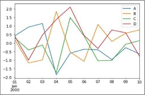
インデックスが日付で構成されている場合は、 gct().autofmt_xdate() 上の図に示すようにx軸をフォーマットします。
を使用して、ある列と別の列をプロットできます。 x そして y キーワード。
プロット方法では、デフォルトの折れ線グラフ以外のいくつかのプロットスタイルを使用できます。これらのメソッドは、kindキーワード引数として提供できます。plot()。これらには以下が含まれます-
- 棒グラフのbarまたはbarh
- ヒストグラムの履歴
- 箱ひげ図のボックス
- エリアプロットの「エリア」
- 散布図の「散布図」
棒グラフ
棒グラフを作成して、棒グラフとは何かを見てみましょう。棒グラフは次の方法で作成できます-
import pandas as pd
import numpy as np
df = pd.DataFrame(np.random.rand(10,4),columns=['a','b','c','d')
df.plot.bar()その output 次のとおりです-
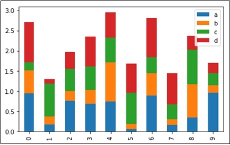
積み上げ棒グラフを作成するには、 pass stacked=True −
import pandas as pd
df = pd.DataFrame(np.random.rand(10,4),columns=['a','b','c','d')
df.plot.bar(stacked=True)その output 次のとおりです-

水平棒グラフを取得するには、 barh 方法−
import pandas as pd
import numpy as np
df = pd.DataFrame(np.random.rand(10,4),columns=['a','b','c','d')
df.plot.barh(stacked=True)その output 次のとおりです-
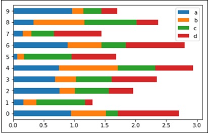
ヒストグラム
ヒストグラムは、 plot.hist()方法。ビンの数を指定できます。
import pandas as pd
import numpy as np
df = pd.DataFrame({'a':np.random.randn(1000)+1,'b':np.random.randn(1000),'c':
np.random.randn(1000) - 1}, columns=['a', 'b', 'c'])
df.plot.hist(bins=20)その output 次のとおりです-
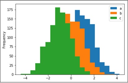
列ごとに異なるヒストグラムをプロットするには、次のコードを使用します-
import pandas as pd
import numpy as np
df=pd.DataFrame({'a':np.random.randn(1000)+1,'b':np.random.randn(1000),'c':
np.random.randn(1000) - 1}, columns=['a', 'b', 'c'])
df.diff.hist(bins=20)その output 次のとおりです-
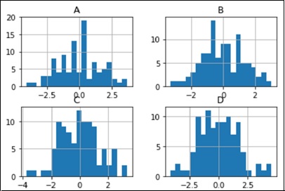
箱ひげ図
箱ひげ図は呼び出して描くことができます Series.box.plot() そして DataFrame.box.plot()、または DataFrame.boxplot() 各列内の値の分布を視覚化します。
たとえば、これは[0,1)の一様確率変数の10回の観測の5回の試行を表す箱ひげ図です。
import pandas as pd
import numpy as np
df = pd.DataFrame(np.random.rand(10, 5), columns=['A', 'B', 'C', 'D', 'E'])
df.plot.box()その output 次のとおりです-

エリアプロット
エリアプロットは、を使用して作成できます Series.plot.area() または DataFrame.plot.area() メソッド。
import pandas as pd
import numpy as np
df = pd.DataFrame(np.random.rand(10, 4), columns=['a', 'b', 'c', 'd'])
df.plot.area()その output 次のとおりです-

散布図
散布図は、を使用して作成できます。 DataFrame.plot.scatter() メソッド。
import pandas as pd
import numpy as np
df = pd.DataFrame(np.random.rand(50, 4), columns=['a', 'b', 'c', 'd'])
df.plot.scatter(x='a', y='b')その output 次のとおりです-
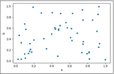
円グラフ
円グラフは、 DataFrame.plot.pie() 方法。
import pandas as pd
import numpy as np
df = pd.DataFrame(3 * np.random.rand(4), index=['a', 'b', 'c', 'd'], columns=['x'])
df.plot.pie(subplots=True)その output 次のとおりです-
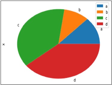
ザ・ Pandas I/O API のようにアクセスされるトップレベルのリーダー関数のセットです pd.read_csv() 通常、Pandasオブジェクトを返します。
テキストファイル(またはフラットファイル)を読み取るための2つの主力機能は次のとおりです。 read_csv() そして read_table()。どちらも同じ解析コードを使用して、表形式のデータをインテリジェントに変換します。DataFrame オブジェクト-
pandas.read_csv(filepath_or_buffer, sep=',', delimiter=None, header='infer',
names=None, index_col=None, usecols=Nonepandas.read_csv(filepath_or_buffer, sep='\t', delimiter=None, header='infer',
names=None, index_col=None, usecols=Noneこれがその方法です csv ファイルデータは次のようになります-
S.No,Name,Age,City,Salary
1,Tom,28,Toronto,20000
2,Lee,32,HongKong,3000
3,Steven,43,Bay Area,8300
4,Ram,38,Hyderabad,3900このデータを次のように保存します temp.csv それに操作を行います。
S.No,Name,Age,City,Salary
1,Tom,28,Toronto,20000
2,Lee,32,HongKong,3000
3,Steven,43,Bay Area,8300
4,Ram,38,Hyderabad,3900このデータを次のように保存します temp.csv それに操作を行います。
read.csv
read.csv csvファイルからデータを読み取り、DataFrameオブジェクトを作成します。
import pandas as pd
df=pd.read_csv("temp.csv")
print dfその output 次のとおりです-
S.No Name Age City Salary
0 1 Tom 28 Toronto 20000
1 2 Lee 32 HongKong 3000
2 3 Steven 43 Bay Area 8300
3 4 Ram 38 Hyderabad 3900カスタムインデックス
これは、csvファイルの列を指定して、を使用してインデックスをカスタマイズします index_col.
import pandas as pd
df=pd.read_csv("temp.csv",index_col=['S.No'])
print dfその output 次のとおりです-
S.No Name Age City Salary
1 Tom 28 Toronto 20000
2 Lee 32 HongKong 3000
3 Steven 43 Bay Area 8300
4 Ram 38 Hyderabad 3900コンバーター
dtype 列の数はdictとして渡すことができます。
import pandas as pd
df = pd.read_csv("temp.csv", dtype={'Salary': np.float64})
print df.dtypesその output 次のとおりです-
S.No int64
Name object
Age int64
City object
Salary float64
dtype: objectデフォルトでは、 dtype 給与列の int、しかし結果はそれを次のように示しています float 型を明示的にキャストしたためです。
したがって、データはfloat −のようになります。
S.No Name Age City Salary
0 1 Tom 28 Toronto 20000.0
1 2 Lee 32 HongKong 3000.0
2 3 Steven 43 Bay Area 8300.0
3 4 Ram 38 Hyderabad 3900.0header_names
names引数を使用してヘッダーの名前を指定します。
import pandas as pd
df=pd.read_csv("temp.csv", names=['a', 'b', 'c','d','e'])
print dfその output 次のとおりです-
a b c d e
0 S.No Name Age City Salary
1 1 Tom 28 Toronto 20000
2 2 Lee 32 HongKong 3000
3 3 Steven 43 Bay Area 8300
4 4 Ram 38 Hyderabad 3900ヘッダー名にはカスタム名が追加されていますが、ファイル内のヘッダーは削除されていません。ここで、ヘッダー引数を使用してそれを削除します。
ヘッダーが最初の行以外の行にある場合は、行番号をヘッダーに渡します。これにより、前の行がスキップされます。
import pandas as pd
df=pd.read_csv("temp.csv",names=['a','b','c','d','e'],header=0)
print dfその output 次のとおりです-
a b c d e
0 S.No Name Age City Salary
1 1 Tom 28 Toronto 20000
2 2 Lee 32 HongKong 3000
3 3 Steven 43 Bay Area 8300
4 4 Ram 38 Hyderabad 3900スキップロー
skiprowsは、指定された行数をスキップします。
import pandas as pd
df=pd.read_csv("temp.csv", skiprows=2)
print dfその output 次のとおりです-
2 Lee 32 HongKong 3000
0 3 Steven 43 Bay Area 8300
1 4 Ram 38 Hyderabad 3900スパースオブジェクトは、特定の値に一致するデータ(NaN /欠落値、ただし任意の値を選択できます)が省略されると、「圧縮」されます。特別なSparseIndexオブジェクトは、データが「スパース化」された場所を追跡します。これは、例でははるかに理にかなっています。すべての標準パンダデータ構造は、to_sparse 方法−
import pandas as pd
import numpy as np
ts = pd.Series(np.random.randn(10))
ts[2:-2] = np.nan
sts = ts.to_sparse()
print stsその output 次のとおりです-
0 -0.810497
1 -1.419954
2 NaN
3 NaN
4 NaN
5 NaN
6 NaN
7 NaN
8 0.439240
9 -1.095910
dtype: float64
BlockIndex
Block locations: array([0, 8], dtype=int32)
Block lengths: array([2, 2], dtype=int32)スパースオブジェクトは、メモリ効率の理由から存在します。
ここで、大きなNA DataFrameがあると仮定して、次のコードを実行します。
import pandas as pd
import numpy as np
df = pd.DataFrame(np.random.randn(10000, 4))
df.ix[:9998] = np.nan
sdf = df.to_sparse()
print sdf.densityその output 次のとおりです-
0.0001スパースオブジェクトは、を呼び出すことで標準のデンスフォームに戻すことができます。 to_dense −
import pandas as pd
import numpy as np
ts = pd.Series(np.random.randn(10))
ts[2:-2] = np.nan
sts = ts.to_sparse()
print sts.to_dense()その output 次のとおりです-
0 -0.810497
1 -1.419954
2 NaN
3 NaN
4 NaN
5 NaN
6 NaN
7 NaN
8 0.439240
9 -1.095910
dtype: float64スパースDtype
スパースデータは、そのデンス表現と同じdtypeを持つ必要があります。現在、float64, int64 そして booldtypesサポートされています。オリジナルに応じてdtype, fill_value default 変化-
float64 − np.nan
int64 − 0
bool −誤り
同じことを理解するために次のコードを実行してみましょう-
import pandas as pd
import numpy as np
s = pd.Series([1, np.nan, np.nan])
print s
s.to_sparse()
print sその output 次のとおりです-
0 1.0
1 NaN
2 NaN
dtype: float64
0 1.0
1 NaN
2 NaN
dtype: float64警告は警告を意味し、落とし穴は目に見えない問題を意味します。
パンダでのIf / Truthステートメントの使用
Pandasは、何かをに変換しようとするとエラーが発生するという厄介な慣習に従います。 bool。これはで起こりますif または when ブール演算を使用して、および、 or、または not。結果がどうあるべきかは明確ではありません。長さがゼロではないので、Trueにする必要がありますか?False値があるのでFalse?はっきりしないので、代わりにパンダはValueError −
import pandas as pd
if pd.Series([False, True, False]):
print 'I am True'その output 次のとおりです-
ValueError: The truth value of a Series is ambiguous.
Use a.empty, a.bool() a.item(),a.any() or a.all().に if状態、それをどうするかは不明です。エラーは、を使用するかどうかを示唆していますNone または any of those。
import pandas as pd
if pd.Series([False, True, False]).any():
print("I am any")その output 次のとおりです-
I am anyブールコンテキストで単一要素のパンダオブジェクトを評価するには、メソッドを使用します .bool() −
import pandas as pd
print pd.Series([True]).bool()その output 次のとおりです-
Trueビット単位のブール
==やのようなビット単位のブール演算子 !=はブール系列を返します。これは、ほとんどの場合、とにかく必要なものです。
import pandas as pd
s = pd.Series(range(5))
print s==4その output 次のとおりです-
0 False
1 False
2 False
3 False
4 True
dtype: boolisin操作
これは、シリーズの各要素が渡された値のシーケンスに正確に含まれているかどうかを示すブールシリーズを返します。
import pandas as pd
s = pd.Series(list('abc'))
s = s.isin(['a', 'c', 'e'])
print sその output 次のとおりです-
0 True
1 False
2 True
dtype: boolインデックスの再作成とixGotcha
多くのユーザーは、 ix indexing capabilities Pandasオブジェクトからデータを選択する簡潔な手段として-
import pandas as pd
import numpy as np
df = pd.DataFrame(np.random.randn(6, 4), columns=['one', 'two', 'three',
'four'],index=list('abcdef'))
print df
print df.ix[['b', 'c', 'e']]その output 次のとおりです-
one two three four
a -1.582025 1.335773 0.961417 -1.272084
b 1.461512 0.111372 -0.072225 0.553058
c -1.240671 0.762185 1.511936 -0.630920
d -2.380648 -0.029981 0.196489 0.531714
e 1.846746 0.148149 0.275398 -0.244559
f -1.842662 -0.933195 2.303949 0.677641
one two three four
b 1.461512 0.111372 -0.072225 0.553058
c -1.240671 0.762185 1.511936 -0.630920
e 1.846746 0.148149 0.275398 -0.244559もちろん、これはこの場合、 reindex 方法−
import pandas as pd
import numpy as np
df = pd.DataFrame(np.random.randn(6, 4), columns=['one', 'two', 'three',
'four'],index=list('abcdef'))
print df
print df.reindex(['b', 'c', 'e'])その output 次のとおりです-
one two three four
a 1.639081 1.369838 0.261287 -1.662003
b -0.173359 0.242447 -0.494384 0.346882
c -0.106411 0.623568 0.282401 -0.916361
d -1.078791 -0.612607 -0.897289 -1.146893
e 0.465215 1.552873 -1.841959 0.329404
f 0.966022 -0.190077 1.324247 0.678064
one two three four
b -0.173359 0.242447 -0.494384 0.346882
c -0.106411 0.623568 0.282401 -0.916361
e 0.465215 1.552873 -1.841959 0.329404一部の人はそれを結論付けるかもしれません ix そして reindexこれに基づいて100%同等です。これは、整数インデックスの場合を除いて当てはまります。たとえば、上記の操作は、次のように表すこともできます。
import pandas as pd
import numpy as np
df = pd.DataFrame(np.random.randn(6, 4), columns=['one', 'two', 'three',
'four'],index=list('abcdef'))
print df
print df.ix[[1, 2, 4]]
print df.reindex([1, 2, 4])その output 次のとおりです-
one two three four
a -1.015695 -0.553847 1.106235 -0.784460
b -0.527398 -0.518198 -0.710546 -0.512036
c -0.842803 -1.050374 0.787146 0.205147
d -1.238016 -0.749554 -0.547470 -0.029045
e -0.056788 1.063999 -0.767220 0.212476
f 1.139714 0.036159 0.201912 0.710119
one two three four
b -0.527398 -0.518198 -0.710546 -0.512036
c -0.842803 -1.050374 0.787146 0.205147
e -0.056788 1.063999 -0.767220 0.212476
one two three four
1 NaN NaN NaN NaN
2 NaN NaN NaN NaN
4 NaN NaN NaN NaNそれを覚えておくことは重要です reindex is strict label indexing only。これは、インデックスに整数と文字列の両方が含まれているなど、病理学的なケースで驚くべき結果をもたらす可能性があります。
多くの潜在的なPandasユーザーはSQLにある程度精通しているため、このページは、パンダを使用してさまざまなSQL操作を実行する方法の例をいくつか提供することを目的としています。
import pandas as pd
url = 'https://raw.github.com/pandasdev/
pandas/master/pandas/tests/data/tips.csv'
tips=pd.read_csv(url)
print tips.head()その output 次のとおりです-
total_bill tip sex smoker day time size
0 16.99 1.01 Female No Sun Dinner 2
1 10.34 1.66 Male No Sun Dinner 3
2 21.01 3.50 Male No Sun Dinner 3
3 23.68 3.31 Male No Sun Dinner 2
4 24.59 3.61 Female No Sun Dinner 4選択する
SQLでは、選択は、選択した列のコンマ区切りリスト(または、すべての列を選択する場合は*)を使用して行われます。
SELECT total_bill, tip, smoker, time
FROM tips
LIMIT 5;Pandasでは、列名のリストをDataFrameに渡すことで列の選択が行われます-
tips[['total_bill', 'tip', 'smoker', 'time']].head(5)プログラム全体をチェックしてみましょう-
import pandas as pd
url = 'https://raw.github.com/pandasdev/
pandas/master/pandas/tests/data/tips.csv'
tips=pd.read_csv(url)
print tips[['total_bill', 'tip', 'smoker', 'time']].head(5)その output 次のとおりです-
total_bill tip smoker time
0 16.99 1.01 No Dinner
1 10.34 1.66 No Dinner
2 21.01 3.50 No Dinner
3 23.68 3.31 No Dinner
4 24.59 3.61 No Dinner列名のリストなしでDataFrameを呼び出すと、すべての列が表示されます(SQLの*と同様)。
どこ
SQLでのフィルタリングは、WHERE句を介して行われます。
SELECT * FROM tips WHERE time = 'Dinner' LIMIT 5;DataFrameは複数の方法でフィルタリングできます。最も直感的なのは、ブールインデックスを使用することです。
tips[tips['time'] == 'Dinner'].head(5)プログラム全体をチェックしてみましょう-
import pandas as pd
url = 'https://raw.github.com/pandasdev/
pandas/master/pandas/tests/data/tips.csv'
tips=pd.read_csv(url)
print tips[tips['time'] == 'Dinner'].head(5)その output 次のとおりです-
total_bill tip sex smoker day time size
0 16.99 1.01 Female No Sun Dinner 2
1 10.34 1.66 Male No Sun Dinner 3
2 21.01 3.50 Male No Sun Dinner 3
3 23.68 3.31 Male No Sun Dinner 2
4 24.59 3.61 Female No Sun Dinner 4上記のステートメントは、一連のTrue / FalseオブジェクトをDataFrameに渡し、すべての行をTrueで返します。
GroupBy
この操作は、データセット全体の各グループのレコード数をフェッチします。たとえば、性別によって残されたヒントの数を取得するクエリ-
SELECT sex, count(*)
FROM tips
GROUP BY sex;パンダに相当するものは-
tips.groupby('sex').size()プログラム全体をチェックしてみましょう-
import pandas as pd
url = 'https://raw.github.com/pandasdev/
pandas/master/pandas/tests/data/tips.csv'
tips=pd.read_csv(url)
print tips.groupby('sex').size()その output 次のとおりです-
sex
Female 87
Male 157
dtype: int64上位N行
SQLは top n rows を使用して LIMIT −
SELECT * FROM tips
LIMIT 5 ;パンダに相当するものは-
tips.head(5)完全な例を確認しましょう-
import pandas as pd
url = 'https://raw.github.com/pandas-dev/pandas/master/pandas/tests/data/tips.csv'
tips=pd.read_csv(url)
tips = tips[['smoker', 'day', 'time']].head(5)
print tipsその output 次のとおりです-
smoker day time
0 No Sun Dinner
1 No Sun Dinner
2 No Sun Dinner
3 No Sun Dinner
4 No Sun Dinnerこれらは、パンダライブラリの前の章で学習したいくつかの基本的な操作です。