PyTorch-선형 회귀

이 장에서는 TensorFlow를 사용한 선형 회귀 구현의 기본 예제에 초점을 맞출 것입니다. 로지스틱 회귀 또는 선형 회귀는 주문 이산 범주 분류를위한 감독 된 기계 학습 접근 방식입니다. 이 장의 목표는 사용자가 예측 변수와 하나 이상의 독립 변수 간의 관계를 예측할 수있는 모델을 구축하는 것입니다.

이 두 변수 사이의 관계는 선형으로 간주됩니다. 즉, y가 종속 변수이고 x가 독립 변수로 간주되면 두 변수의 선형 회귀 관계는 아래에 언급 된 방정식과 같습니다.

Y = Ax+b

다음으로, 우리는 아래에 주어진 두 가지 중요한 개념을 이해할 수있는 선형 회귀 알고리즘을 설계 할 것입니다.

비용 함수
경사 하강 법 알고리즘

선형 회귀의 개략적 표현은 아래에 언급되어 있습니다.

결과 해석

$$ Y = ax + b $$

의 가치 a 경사입니다.
의 가치 b 이다 y − intercept.
r 이다 correlation coefficient.
r² 이다 correlation coefficient.

선형 회귀 방정식의 그래픽보기는 다음과 같습니다.

다음 단계는 PyTorch를 사용하여 선형 회귀를 구현하는 데 사용됩니다-

1 단계

아래 코드를 사용하여 PyTorch에서 선형 회귀를 만드는 데 필요한 패키지를 가져옵니다.

import numpy as np
import matplotlib.pyplot as plt
from matplotlib.animation import FuncAnimation
import seaborn as sns
import pandas as pd
%matplotlib inline

sns.set_style(style = 'whitegrid')
plt.rcParams["patch.force_edgecolor"] = True

2 단계

아래와 같이 사용 가능한 데이터 세트로 단일 훈련 세트를 만듭니다.

m = 2 # slope
c = 3 # interceptm = 2 # slope
c = 3 # intercept
x = np.random.rand(256)

noise = np.random.randn(256) / 4

y = x * m + c + noise

df = pd.DataFrame()
df['x'] = x
df['y'] = y

sns.lmplot(x ='x', y ='y', data = df)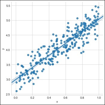

3 단계

아래에 언급 된대로 PyTorch 라이브러리로 선형 회귀를 구현하십시오.

import torch
import torch.nn as nn
from torch.autograd import Variable
x_train = x.reshape(-1, 1).astype('float32')
y_train = y.reshape(-1, 1).astype('float32')

class LinearRegressionModel(nn.Module):
   def __init__(self, input_dim, output_dim):
      super(LinearRegressionModel, self).__init__()
      self.linear = nn.Linear(input_dim, output_dim)

   def forward(self, x):
      out = self.linear(x)
      return out
input_dim = x_train.shape[1]
output_dim = y_train.shape[1]
input_dim, output_dim(1, 1)
model = LinearRegressionModel(input_dim, output_dim)
criterion = nn.MSELoss()
[w, b] = model.parameters()

def get_param_values():
   return w.data[0][0], b.data[0]

def plot_current_fit(title = ""):
plt.figure(figsize = (12,4))
plt.title(title)
plt.scatter(x, y, s = 8)
w1 = w.data[0][0]
b1 = b.data[0]
x1 = np.array([0., 1.])
y1 = x1 * w1 + b1
plt.plot(x1, y1, 'r', label = 'Current Fit ({:.3f}, {:.3f})'.format(w1, b1))
plt.xlabel('x (input)')
plt.ylabel('y (target)')
plt.legend()
plt.show()
plot_current_fit('Before training')

생성 된 플롯은 다음과 같습니다.