Automata Theory - คู่มือฉบับย่อ
Automata - มันคืออะไร?
คำว่า "Automata" มาจากคำภาษากรีก "αὐτόματα" ซึ่งแปลว่า "การแสดงด้วยตนเอง" หุ่นยนต์ (Automata ในรูปพหูพจน์) เป็นอุปกรณ์คอมพิวเตอร์ที่ขับเคลื่อนด้วยตัวเองแบบนามธรรมซึ่งเป็นไปตามลำดับการทำงานที่กำหนดไว้ล่วงหน้าโดยอัตโนมัติ
หุ่นยนต์ที่มีสถานะจำนวน จำกัด เรียกว่า a Finite Automaton (FA) หรือ Finite State Machine (FSM).
คำจำกัดความอย่างเป็นทางการของ Finite Automaton
หุ่นยนต์สามารถแสดงด้วย 5-tuple (Q, ∑, δ, q 0 , F) โดยที่ -
Q เป็นชุดของรัฐที่ จำกัด
∑ เป็นชุดสัญลักษณ์ที่ จำกัด เรียกว่า alphabet ของหุ่นยนต์
δ คือฟังก์ชันการเปลี่ยนแปลง
q0คือสถานะเริ่มต้นจากการที่อินพุตใด ๆ ถูกประมวลผล (q 0 ∈ Q)
F คือชุดของสถานะสุดท้าย / สถานะของ Q (F ⊆ Q)
คำศัพท์ที่เกี่ยวข้อง
ตัวอักษร
Definition - อ alphabet คือชุดสัญลักษณ์ที่ จำกัด
Example - ∑ = {a, b, c, d} คือ alphabet set โดยที่ 'a', 'b', 'c' และ 'd' อยู่ symbols.
สตริง
Definition - ก string เป็นลำดับ จำกัด ของสัญลักษณ์ที่นำมาจาก ∑
Example - 'cabcad' เป็นสตริงที่ถูกต้องในชุดตัวอักษร ∑ = {a, b, c, d}
ความยาวของสตริง
Definition- เป็นจำนวนสัญลักษณ์ที่มีอยู่ในสตริง (แสดงโดย|S|).
Examples -
ถ้า S = 'cabcad', | S | = 6
ถ้า | S | = 0 เรียกว่าไฟล์ empty string (แสดงโดย λ หรือ ε)
คลีนสตาร์
Definition - ดาวคลีน ∑*เป็นตัวดำเนินการยูนารีในชุดของสัญลักษณ์หรือสตริง ∑ซึ่งจะให้ชุดสตริงที่เป็นไปได้ทั้งหมดที่เป็นไปได้ไม่สิ้นสุด ∑ ได้แก่ λ.
Representation- ∑ * = ∑ 0 ∪ ∑ 1 ∪ ∑ 2 ∪……. โดยที่ ∑ pคือเซตของสตริงความยาวที่เป็นไปได้ทั้งหมด p
Example - ถ้า ∑ = {a, b}, ∑ * = {λ, a, b, aa, ab, ba, bb, ……… .. }
คลีนปิด / พลัส
Definition - ชุด ∑+ คือเซตที่ไม่สิ้นสุดของสตริงที่เป็นไปได้ทั้งหมดของความยาวที่เป็นไปได้ทั้งหมดที่มากกว่า ∑ ไม่รวมλ
Representation- ∑ + = ∑ 1 ∪ ∑ 2 ∪ ∑ 3 ∪…….
∑ + = ∑ * - {λ}
Example- ถ้า ∑ = {a, b}, ∑ + = {a, b, aa, ab, ba, bb, ……… .. }
ภาษา
Definition- ภาษาเป็นส่วนย่อยของ ∑ * สำหรับตัวอักษรบางตัว ∑ สามารถ จำกัด หรือไม่มีที่สิ้นสุด
Example - ถ้าภาษาใช้สตริงที่เป็นไปได้ทั้งหมดที่มีความยาว 2 มากกว่า ∑ = {a, b} แล้ว L = {ab, aa, ba, bb}
Finite Automaton สามารถแบ่งออกเป็นสองประเภท -
- กำหนด Finite Automaton (DFA)
- Finite Automaton แบบไม่กำหนด (NDFA / NFA)
กำหนด Finite Automaton (DFA)
ใน DFA สำหรับสัญลักษณ์อินพุตแต่ละสัญลักษณ์สามารถกำหนดสถานะที่เครื่องจักรจะเคลื่อนที่ได้ ดังนั้นจึงเรียกว่าDeterministic Automaton. เนื่องจากมีสถานะจำนวน จำกัด จึงเรียกเครื่องDeterministic Finite Machine หรือ Deterministic Finite Automaton.
คำจำกัดความอย่างเป็นทางการของ DFA
DFA สามารถแสดงด้วย 5-tuple (Q, ∑, δ, q 0 , F) โดยที่ -
Q เป็นชุดของรัฐที่ จำกัด
∑ เป็นชุดสัญลักษณ์ จำกัด ที่เรียกว่าตัวอักษร
δ คือฟังก์ชันการเปลี่ยนโดยที่δ: Q × ∑ → Q
q0คือสถานะเริ่มต้นจากการที่อินพุตใด ๆ ถูกประมวลผล (q 0 ∈ Q)
F คือชุดของสถานะสุดท้าย / สถานะของ Q (F ⊆ Q)
การแสดงกราฟิกของ DFA
DFA แสดงด้วยกราฟที่เรียกว่า state diagram.
- จุดยอดแสดงถึงสถานะ
- ส่วนโค้งที่มีป้ายกำกับด้วยอักษรอินพุตแสดงการเปลี่ยน
- สถานะเริ่มต้นแสดงด้วยส่วนโค้งขาเข้าเดี่ยวที่ว่างเปล่า
- สถานะสุดท้ายถูกระบุด้วยวงกลมสองวง
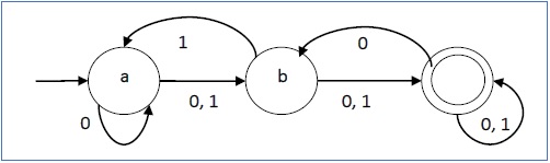
ตัวอย่าง
ให้หุ่นยนต์ จำกัด กำหนดเป็น→
- ถาม = {a, b, c},
- ∑ = {0, 1},
- q 0 = {a}
- F = {c} และ
ฟังก์ชันการเปลี่ยนδดังแสดงในตารางต่อไปนี้ -
| สถานะปัจจุบัน | สถานะถัดไปสำหรับอินพุต 0 | สถานะถัดไปสำหรับอินพุต 1 |
|---|---|---|
| a | ก | ข |
| b | ค | ก |
| c | ข | ค |
การแสดงกราฟิกจะเป็นดังนี้ -

ใน NDFA สำหรับสัญลักษณ์อินพุตเฉพาะเครื่องสามารถย้ายไปยังสถานะใดก็ได้ในเครื่องรวมกัน กล่าวอีกนัยหนึ่งไม่สามารถระบุสถานะที่แน่นอนที่เครื่องจักรเคลื่อนที่ได้ ดังนั้นจึงเรียกว่าNon-deterministic Automaton. เนื่องจากมีจำนวนสถานะ จำกัด เครื่องจึงถูกเรียกNon-deterministic Finite Machine หรือ Non-deterministic Finite Automaton.
คำจำกัดความอย่างเป็นทางการของ NDFA
NDFA สามารถแสดงด้วย 5-tuple (Q, ∑, δ, q 0 , F) โดยที่ -
Q เป็นชุดของรัฐที่ จำกัด
∑ เป็นชุดสัญลักษณ์ จำกัด ที่เรียกว่าตัวอักษร
δคือฟังก์ชันการเปลี่ยนโดยที่δ: Q × ∑ → 2 Q
(ที่นี่ชุดกำลังของ Q (2 Q ) ถูกนำมาใช้เนื่องจากในกรณีของ NDFA จากสถานะการเปลี่ยนอาจเกิดขึ้นกับการรวมกันของสถานะ Q ใด ๆ )
q0คือสถานะเริ่มต้นจากการที่อินพุตใด ๆ ถูกประมวลผล (q 0 ∈ Q)
F คือชุดของสถานะสุดท้าย / สถานะของ Q (F ⊆ Q)
การแสดงกราฟิกของ NDFA: (เหมือนกับ DFA)
NDFA แสดงด้วย digraphs เรียกว่า state diagram
- จุดยอดแสดงถึงสถานะ
- ส่วนโค้งที่มีป้ายกำกับด้วยอักษรอินพุตแสดงการเปลี่ยน
- สถานะเริ่มต้นแสดงด้วยส่วนโค้งขาเข้าเดี่ยวที่ว่างเปล่า
- สถานะสุดท้ายถูกระบุด้วยวงกลมสองวง
Example
ให้หุ่นยนต์ จำกัด ที่ไม่ใช่ปัจจัยกำหนดเป็น→
- ถาม = {a, b, c}
- ∑ = {0, 1}
- q 0 = {a}
- F = {c}
ฟังก์ชันการเปลี่ยนแปลงδดังแสดงด้านล่าง -
| สถานะปัจจุบัน | สถานะถัดไปสำหรับอินพุต 0 | สถานะถัดไปสำหรับอินพุต 1 |
|---|---|---|
| ก | ก, ข | ข |
| ข | ค | ก, ค |
| ค | ข, ค | ค |
การแสดงกราฟิกจะเป็นดังนี้ -
DFA กับ NDFA
ตารางต่อไปนี้แสดงความแตกต่างระหว่าง DFA และ NDFA
| DFA | NDFA |
|---|---|
| การเปลี่ยนจากสถานะเป็นสถานะถัดไปเฉพาะสำหรับสัญลักษณ์อินพุตแต่ละรายการ ดังนั้นจึงเรียกว่าดีเทอร์มินิสติก | การเปลี่ยนจากสถานะสามารถเป็นสถานะถัดไปได้หลายสถานะสำหรับสัญลักษณ์อินพุตแต่ละตัว ดังนั้นมันจะเรียกว่าไม่ใช่กำหนด |
| ไม่เห็นการเปลี่ยนสตริงว่างใน DFA | NDFA อนุญาตให้เปลี่ยนสตริงว่าง |
| อนุญาตให้ย้อนรอยใน DFA | ใน NDFA การย้อนรอยไม่สามารถทำได้เสมอไป |
| ต้องใช้พื้นที่มากขึ้น | ต้องการพื้นที่น้อย |
| DFA ยอมรับสตริงหากส่งผ่านไปยังสถานะสุดท้าย | NDFA ยอมรับสตริงหากการเปลี่ยนแปลงที่เป็นไปได้อย่างน้อยหนึ่งรายการสิ้นสุดในสถานะสุดท้าย |
ตัวรับตัวแยกประเภทและตัวแปลงสัญญาณ
ผู้รับ (Recognizer)
หุ่นยนต์ที่คำนวณฟังก์ชันบูลีนเรียกว่าไฟล์ acceptor. สถานะทั้งหมดของตัวรับคือการยอมรับหรือปฏิเสธอินพุตที่ให้ไว้
ลักษณนาม
ก classifier มีสถานะสุดท้ายมากกว่าสองสถานะและจะให้เอาต์พุตเดียวเมื่อสิ้นสุด
ทรานสดิวเซอร์
หุ่นยนต์ที่สร้างเอาต์พุตตามอินพุตปัจจุบันและ / หรือสถานะก่อนหน้านี้เรียกว่า a transducer. ทรานสดิวเซอร์สามารถมีได้สองประเภท -
Mealy Machine - เอาต์พุตขึ้นอยู่กับสถานะปัจจุบันและอินพุตปัจจุบัน
Moore Machine - เอาต์พุตขึ้นอยู่กับสถานะปัจจุบันเท่านั้น
การยอมรับโดย DFA และ NDFA
DFA / NDFA ยอมรับสตริงหาก DFA / NDFA เริ่มต้นที่สถานะเริ่มต้นจะสิ้นสุดในสถานะยอมรับ (สถานะสุดท้ายใด ๆ ) หลังจากอ่านสตริงทั้งหมด
DFA / NDFA ยอมรับสตริง S (Q, ∑, δ, q 0 , F), iff
δ*(q0, S) ∈ F
ภาษา L ยอมรับโดย DFA / NDFA คือ
{S | S ∈ ∑* and δ*(q0, S) ∈ F}
DFA / NDFA ไม่ยอมรับสตริง S ′(Q, ∑, δ, q 0 , F), iff
δ*(q0, S′) ∉ F
ภาษา L ′ไม่ยอมรับโดย DFA / NDFA (ส่วนเสริมของภาษาที่ยอมรับ L) คือ
{S | S ∈ ∑* and δ*(q0, S) ∉ F}
Example
ให้เราพิจารณา DFA ที่แสดงในรูปที่ 1.3 จาก DFA สามารถรับสตริงที่ยอมรับได้

สตริงที่ DFA ยอมรับข้างต้น: {0, 00, 11, 010, 101, ........... }
DFA ข้างต้นไม่ยอมรับสตริง: {1, 011, 111, ........ }
คำชี้แจงปัญหา
ปล่อย X = (Qx, ∑, δx, q0, Fx)เป็น NDFA ซึ่งยอมรับภาษา L (X) เราต้องออกแบบ DFA ที่เทียบเท่าY = (Qy, ∑, δy, q0, Fy) ดังนั้น L(Y) = L(X). ขั้นตอนต่อไปนี้แปลง NDFA เป็น DFA ที่เทียบเท่า -
อัลกอริทึม
Input - NDFA
Output - DFA ที่เทียบเท่า
Step 1 - สร้างตารางสถานะจาก NDFA ที่กำหนด
Step 2 - สร้างตารางสถานะว่างภายใต้ตัวอักษรอินพุตที่เป็นไปได้สำหรับ DFA ที่เทียบเท่า
Step 3 - ทำเครื่องหมายสถานะเริ่มต้นของ DFA ด้วย q0 (เหมือนกับ NDFA)
Step 4- ค้นหาการรวมกันของ States {Q 0 , Q 1 , ... , Q n } สำหรับตัวอักษรที่ป้อนได้แต่ละตัว
Step 5 - ทุกครั้งที่เราสร้างสถานะ DFA ใหม่ภายใต้คอลัมน์ตัวอักษรอินพุตเราจะต้องใช้ขั้นตอนที่ 4 อีกครั้งมิฉะนั้นให้ไปที่ขั้นตอนที่ 6
Step 6 - รัฐที่มีสถานะสุดท้ายของ NDFA เป็นสถานะสุดท้ายของ DFA ที่เทียบเท่า
ตัวอย่าง
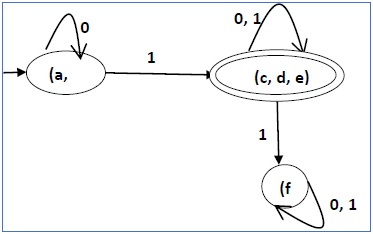
ให้เราพิจารณา NDFA ที่แสดงในรูปด้านล่าง

| q | δ (q, 0) | δ (q, 1) |
|---|---|---|
| ก | {a, b, c, d, e} | {d, e} |
| ข | {ค} | {e} |
| ค | ∅ | {b} |
| ง | {e} | ∅ |
| จ | ∅ | ∅ |
เมื่อใช้อัลกอริทึมข้างต้นเราจะพบ DFA ที่เทียบเท่า ตารางสถานะของ DFA แสดงอยู่ด้านล่าง
| q | δ (q, 0) | δ (q, 1) |
|---|---|---|
| [a] | [a, b, c, d, e] | [d, e] |
| [a, b, c, d, e] | [a, b, c, d, e] | [b, d, e] |
| [d, e] | [e] | ∅ |
| [b, d, e] | [c, e] | [e] |
| [e] | ∅ | ∅ |
| [c, e] | ∅ | [b] |
| [b] | [ค] | [e] |
| [ค] | ∅ | [b] |
แผนภาพสถานะของ DFA มีดังนี้ -

การย่อขนาด DFA โดยใช้ Myhill-Nerode Theorem
อัลกอริทึม
Input - DFA
Output - ย่อขนาด DFA
Step 1- วาดตารางสำหรับทุกคู่ของสถานะ (Q i , Q j ) ไม่จำเป็นต้องเชื่อมต่อโดยตรง [ทั้งหมดจะไม่มีเครื่องหมายในตอนแรก]
Step 2- พิจารณาทุกคู่สถานะ (Q i , Q j ) ใน DFA โดยที่ Q i ∈ F และ Q j ∉ F หรือกลับกันแล้วทำเครื่องหมาย [ที่นี่ F คือชุดของสถานะสุดท้าย]
Step 3 - ทำซ้ำขั้นตอนนี้จนกว่าเราจะไม่สามารถทำเครื่องหมายสถานะได้อีกต่อไป -
หากมีคู่ที่ไม่มีเครื่องหมาย (Q i , Q j ) ให้ทำเครื่องหมายว่าคู่ {δ (Q i , A), δ (Q i , A)} ถูกทำเครื่องหมายไว้สำหรับตัวอักษรอินพุตบางตัว
Step 4- รวมคู่ที่ไม่มีเครื่องหมายทั้งหมด (Q i , Q j ) และทำให้เป็นสถานะเดียวใน DFA ที่ลดลง
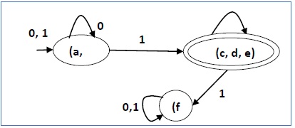
ตัวอย่าง
ให้เราใช้อัลกอริทึม 2 เพื่อย่อ DFA ที่แสดงด้านล่าง

Step 1 - เราวาดตารางสำหรับทุกคู่ของรัฐ
| ก | ข | ค | ง | จ | ฉ | |
| ก | ||||||
| ข | ||||||
| ค | ||||||
| ง | ||||||
| จ | ||||||
| ฉ |
Step 2 - เราทำเครื่องหมายคู่สถานะ
| ก | ข | ค | ง | จ | ฉ | |
| ก | ||||||
| ข | ||||||
| ค | ✔ | ✔ | ||||
| ง | ✔ | ✔ | ||||
| จ | ✔ | ✔ | ||||
| ฉ | ✔ | ✔ | ✔ |
Step 3- เราจะพยายามทำเครื่องหมายคู่สถานะด้วยเครื่องหมายถูกสีเขียวตามสกรรมกริยา ถ้าเราใส่ 1 เพื่อระบุ 'a' และ 'f' มันจะไปที่สถานะ 'c' และ 'f' ตามลำดับ (c, f) ถูกทำเครื่องหมายไว้แล้วดังนั้นเราจะทำเครื่องหมายคู่ (a, f) ตอนนี้เราป้อน 1 เพื่อระบุ 'b' และ 'f'; มันจะไปที่สถานะ 'd' และ 'f' ตามลำดับ (d, f) ถูกทำเครื่องหมายไว้แล้วดังนั้นเราจะทำเครื่องหมายคู่ (b, f)
| ก | ข | ค | ง | จ | ฉ | |
| ก | ||||||
| ข | ||||||
| ค | ✔ | ✔ | ||||
| ง | ✔ | ✔ | ||||
| จ | ✔ | ✔ | ||||
| ฉ | ✔ | ✔ | ✔ | ✔ | ✔ |
หลังจากขั้นตอนที่ 3 เรามีชุดค่าผสมของสถานะ {a, b} {c, d} {c, e} {d, e} ที่ไม่มีเครื่องหมาย
เราสามารถรวม {c, d} {c, e} {d, e} เป็น {c, d, e}
ดังนั้นเราจึงมีสองสถานะรวมกันคือ - {a, b} และ {c, d, e}
ดังนั้น DFA ที่ย่อขนาดสุดท้ายจะมีสามสถานะ {f}, {a, b} และ {c, d, e}
การย่อขนาด DFA โดยใช้ทฤษฎีบทความเท่าเทียมกัน
หาก X และ Y เป็นสองสถานะใน DFA เราสามารถรวมสองสถานะนี้เป็น {X, Y} ได้หากไม่สามารถแยกแยะได้ สองสถานะสามารถแยกแยะได้หากมีอย่างน้อยหนึ่งสตริง S เช่นหนึ่งในδ (X, S) และδ (Y, S) ยอมรับและอีกสถานะหนึ่งไม่ยอมรับ ดังนั้น DFA จึงมีน้อยมากก็ต่อเมื่อทุกรัฐสามารถแยกแยะได้
อัลกอริทึม 3
Step 1 - ทุกรัฐ Q แบ่งออกเป็นสองพาร์ติชัน - final states และ non-final states และแสดงโดย P0. ทุกรัฐในพาร์ทิชัน 0 THเทียบเท่า ใช้เคาน์เตอร์k และเริ่มต้นด้วย 0
Step 2- เพิ่ม k โดย 1 สำหรับแต่ละพาร์ติชันใน P kให้แบ่งสถานะใน P kออกเป็นสองพาร์ติชั่นถ้าแยกได้ k สองสถานะภายในพาร์ติชัน X และ Y นี้สามารถแยกความแตกต่าง k ได้หากมีอินพุตS ดังนั้น δ(X, S) และ δ(Y, S) เป็น (k-1) - แยกแยะได้
Step 3- หาก P k ≠ P k-1ให้ทำซ้ำขั้นตอนที่ 2 มิฉะนั้นไปที่ขั้นตอนที่ 4
Step 4- นวด k THชุดเทียบเท่าและทำให้พวกเขารัฐใหม่ของการลดลง DFA
ตัวอย่าง
ให้เราพิจารณา DFA ต่อไปนี้ -

| q | δ (q, 0) | δ (q, 1) |
|---|---|---|
| ก | ข | ค |
| ข | ก | ง |
| ค | จ | ฉ |
| ง | จ | ฉ |
| จ | จ | ฉ |
| ฉ | ฉ | ฉ |
ให้เราใช้อัลกอริทึมข้างต้นกับ DFA ข้างต้น -
- P 0 = {(c, d, e), (a, b, f)}
- ป1 = {(c, d, e), (a, b), (f)}
- ป2 = {(c, d, e), (a, b), (f)}
ดังนั้น P 1 = P 2
DFA ที่ลดลงมีสามสถานะ DFA ที่ลดลงมีดังนี้ -
| ถาม | δ (q, 0) | δ (q, 1) |
|---|---|---|
| (ก, ข) | (ก, ข) | (ค, ง, จ) |
| (ค, ง, จ) | (ค, ง, จ) | (ฉ) |
| (ฉ) | (ฉ) | (ฉ) |
Finite automata อาจมีเอาต์พุตที่สอดคล้องกับการเปลี่ยนแปลงแต่ละครั้ง มีเครื่องจักรสถานะ จำกัด สองประเภทที่สร้างเอาต์พุต -
- เครื่องแป้ง
- เครื่องมัว
เครื่องแป้ง
Mealy Machine เป็น FSM ซึ่งเอาต์พุตขึ้นอยู่กับสถานะปัจจุบันและอินพุตปัจจุบัน
สามารถอธิบายได้ด้วย 6 ทูเปิล (Q, ∑, O, δ, X, q 0 ) โดยที่ -
Q เป็นชุดของรัฐที่ จำกัด
∑ เป็นชุดสัญลักษณ์ จำกัด ที่เรียกว่าตัวอักษรอินพุต
O เป็นชุดสัญลักษณ์ จำกัด ที่เรียกว่าอักษรเอาต์พุต
δ คือฟังก์ชั่นการเปลี่ยนอินพุตโดยที่δ: Q × ∑ → Q
X คือฟังก์ชันการเปลี่ยนเอาต์พุตโดยที่ X: Q × ∑ → O
q0คือสถานะเริ่มต้นจากการที่อินพุตใด ๆ ถูกประมวลผล (q 0 ∈ Q)
ตารางสถานะของเครื่อง Mealy แสดงไว้ด้านล่าง -
| สถานะปัจจุบัน | ชาติหน้า | |||
|---|---|---|---|---|
| อินพุต = 0 | อินพุต = 1 | |||
| สถานะ | เอาต์พุต | สถานะ | เอาต์พุต | |
| →ก | ข | x 1 | ค | x 1 |
| ข | ข | x 2 | ง | x 3 |
| ค | ง | x 3 | ค | x 1 |
| ง | ง | x 3 | ง | x 2 |
แผนภาพสถานะของ Mealy Machine ข้างต้นคือ -

มัวร์แมชชีน
Moore machine เป็น FSM ซึ่งเอาต์พุตขึ้นอยู่กับสถานะปัจจุบันเท่านั้น
เครื่อง Moore สามารถอธิบายได้ด้วย 6 tuple (Q, ∑, O, δ, X, q 0 ) โดยที่ -
Q เป็นชุดของรัฐที่ จำกัด
∑ เป็นชุดสัญลักษณ์ จำกัด ที่เรียกว่าตัวอักษรอินพุต
O เป็นชุดสัญลักษณ์ จำกัด ที่เรียกว่าอักษรเอาต์พุต
δ คือฟังก์ชั่นการเปลี่ยนอินพุตโดยที่δ: Q × ∑ → Q
X คือฟังก์ชันการเปลี่ยนเอาต์พุตโดยที่ X: Q → O
q0คือสถานะเริ่มต้นจากการที่อินพุตใด ๆ ถูกประมวลผล (q 0 ∈ Q)
ตารางสถานะของ Moore Machine แสดงไว้ด้านล่าง -
| สถานะปัจจุบัน | รัฐถัดไป | เอาต์พุต | |
|---|---|---|---|
| อินพุต = 0 | อินพุต = 1 | ||
| →ก | ข | ค | x 2 |
| ข | ข | ง | x 1 |
| ค | ค | ง | x 2 |
| ง | ง | ง | x 3 |
แผนภาพสถานะของ Moore Machine ข้างต้นคือ -

Mealy Machine กับ Moore Machine
ตารางต่อไปนี้เน้นประเด็นที่ทำให้ Mealy Machine แตกต่างจาก Moore Machine
| เครื่องแป้ง | มัวร์แมชชีน |
|---|---|
| เอาต์พุตขึ้นอยู่กับสถานะปัจจุบันและอินพุตปัจจุบัน | ผลลัพธ์ขึ้นอยู่กับสถานะปัจจุบันเท่านั้น |
| โดยทั่วไปจะมีสถานะน้อยกว่า Moore Machine | โดยทั่วไปจะมีสถานะมากกว่า Mealy Machine |
| ค่าของฟังก์ชันเอาต์พุตเป็นฟังก์ชันของการเปลี่ยนและการเปลี่ยนแปลงเมื่อตรรกะอินพุตในสถานะปัจจุบันเสร็จสิ้น | ค่าของฟังก์ชันเอาต์พุตเป็นฟังก์ชันของสถานะปัจจุบันและการเปลี่ยนแปลงที่ขอบนาฬิกาเมื่อใดก็ตามที่เกิดการเปลี่ยนแปลงสถานะ |
| เครื่องจักร Mealy ตอบสนองต่ออินพุตได้เร็วขึ้น โดยทั่วไปจะตอบสนองในวงจรนาฬิกาเดียวกัน | ในเครื่องมัวร์จำเป็นต้องใช้ตรรกะมากขึ้นในการถอดรหัสเอาต์พุตซึ่งส่งผลให้วงจรล่าช้ามากขึ้น โดยทั่วไปจะตอบสนองหนึ่งรอบนาฬิกาในภายหลัง |
Moore Machine ไปยัง Mealy Machine
อัลกอริทึม 4
Input - เครื่องมัวร์
Output - เครื่องแป้ง
Step 1 - ใช้รูปแบบตารางการเปลี่ยน Mealy Machine ที่ว่างเปล่า
Step 2 - คัดลอกสถานะการเปลี่ยนแปลงของ Moore Machine ทั้งหมดลงในรูปแบบตารางนี้
Step 3- ตรวจสอบสถานะปัจจุบันและผลลัพธ์ที่เกี่ยวข้องในตารางสถานะของ Moore Machine ถ้าสำหรับเอาต์พุตสถานะ Q iคือ m ให้คัดลอกลงในคอลัมน์เอาต์พุตของตารางสถานะ Mealy Machine ที่ใดก็ตามที่ Q iปรากฏในสถานะถัดไป
ตัวอย่าง
ให้เราพิจารณาเครื่อง Moore ดังต่อไปนี้ -
| สถานะปัจจุบัน | รัฐถัดไป | เอาต์พุต | |
|---|---|---|---|
| a = 0 | a = 1 | ||
| →ก | ง | ข | 1 |
| ข | ก | ง | 0 |
| ค | ค | ค | 0 |
| ง | ข | ก | 1 |
ตอนนี้เราใช้ Algorithm 4 เพื่อแปลงเป็น Mealy Machine
Step 1 & 2 -
| สถานะปัจจุบัน | รัฐถัดไป | |||
|---|---|---|---|---|
| a = 0 | a = 1 | |||
| สถานะ | เอาต์พุต | สถานะ | เอาต์พุต | |
| →ก | ง | ข | ||
| ข | ก | ง | ||
| ค | ค | ค | ||
| ง | ข | ก | ||
Step 3 -
| สถานะปัจจุบัน | รัฐถัดไป | |||
|---|---|---|---|---|
| a = 0 | a = 1 | |||
| สถานะ | เอาต์พุต | สถานะ | เอาต์พุต | |
| => ก | ง | 1 | ข | 0 |
| ข | ก | 1 | ง | 1 |
| ค | ค | 0 | ค | 0 |
| ง | ข | 0 | ก | 1 |
Mealy Machine ไปยัง Moore Machine
อัลกอริทึม 5
Input - เครื่องแป้ง
Output - เครื่องมัวร์
Step 1- คำนวณจำนวนเอาต์พุตที่แตกต่างกันสำหรับแต่ละสถานะ (Q i ) ที่มีอยู่ในตารางสถานะของเครื่อง Mealy
Step 2- ถ้าหากผลของฉีเหมือนกันคัดลอกรัฐ Q ฉัน หากมี n เอาต์พุตที่แตกต่างกันให้แบ่ง Q iเป็น n สถานะเป็น Q ในที่ใดn = 0, 1, 2 .......
Step 3 - หากเอาต์พุตของสถานะเริ่มต้นเป็น 1 ให้ใส่สถานะเริ่มต้นใหม่ที่จุดเริ่มต้นซึ่งให้เอาต์พุต 0
ตัวอย่าง
ให้เราพิจารณา Mealy Machine ต่อไปนี้ -
| สถานะปัจจุบัน | รัฐถัดไป | |||
|---|---|---|---|---|
| a = 0 | a = 1 | |||
| รัฐถัดไป | เอาต์พุต | รัฐถัดไป | เอาต์พุต | |
| →ก | ง | 0 | ข | 1 |
| ข | ก | 1 | ง | 0 |
| ค | ค | 1 | ค | 0 |
| ง | ข | 0 | ก | 1 |
ที่นี่สถานะ 'a' และ 'd' ให้ผลลัพธ์เพียง 1 และ 0 ตามลำดับดังนั้นเราจึงคงสถานะ 'a' และ 'd' แต่สถานะ 'b' และ 'c' ให้ผลลัพธ์ที่แตกต่างกัน (1 และ 0) ดังนั้นเราจึงแบ่งb เป็น b0, b1 และ c เป็น c0, c1.
| สถานะปัจจุบัน | รัฐถัดไป | เอาต์พุต | |
|---|---|---|---|
| a = 0 | a = 1 | ||
| →ก | ง | ข1 | 1 |
| ข0 | ก | ง | 0 |
| ข1 | ก | ง | 1 |
| ค0 | ค1 | ค0 | 0 |
| ค1 | ค1 | ค0 | 1 |
| ง | ข0 | ก | 0 |
n ความหมายทางวรรณกรรมของศัพท์ไวยากรณ์แสดงถึงกฎวากยสัมพันธ์สำหรับการสนทนาในภาษาธรรมชาติ ภาษาศาสตร์ได้พยายามกำหนดไวยากรณ์ตั้งแต่เริ่มใช้ภาษาธรรมชาติเช่นอังกฤษสันสกฤตจีนกลางเป็นต้น
ทฤษฎีของภาษาที่เป็นทางการพบว่าสามารถนำไปใช้ได้อย่างกว้างขวางในสาขาวิทยาศาสตร์คอมพิวเตอร์ Noam Chomsky ให้แบบจำลองทางคณิตศาสตร์ของไวยากรณ์ในปีพ. ศ. 2499 ซึ่งมีผลบังคับใช้สำหรับการเขียนภาษาคอมพิวเตอร์
ไวยากรณ์
ไวยากรณ์ G สามารถเขียนอย่างเป็นทางการเป็น 4-tuple (N, T, S, P) โดยที่ -
N หรือ VN คือชุดของตัวแปรหรือสัญลักษณ์ที่ไม่ใช่ขั้ว
T หรือ ∑ คือชุดสัญลักษณ์ Terminal
S เป็นตัวแปรพิเศษที่เรียกว่าสัญลักษณ์ Start, S ∈ N
Pคือกฎการผลิตสำหรับเทอร์มินัลและไม่ใช่เทอร์มินัล กฎการผลิตมีรูปแบบα→βที่αและβสตริงวีN ∪Σและอย่างน้อยหนึ่งสัญลักษณ์ของαเป็น V N
ตัวอย่าง
ไวยากรณ์ G1 -
({S, A, B}, {a, b}, S, {S → AB, A → a, B → b})
ที่นี่
S, A, และ B เป็นสัญลักษณ์ที่ไม่ใช่ขั้ว
a และ b คือสัญลักษณ์ Terminal
S คือสัญลักษณ์เริ่ม S ∈ N
โปรดักชั่น, P : S → AB, A → a, B → b
ตัวอย่าง
ไวยากรณ์ G2 -
(({S, A}, {a, b}, S, {S → aAb, aA → aaAb, A →ε})
ที่นี่
S และ A เป็นสัญลักษณ์ที่ไม่ใช่ขั้ว
a และ b คือสัญลักษณ์ Terminal
ε เป็นสตริงว่าง
S คือสัญลักษณ์เริ่ม S ∈ N
การผลิต P : S → aAb, aA → aaAb, A → ε
รากศัพท์จากไวยากรณ์
สตริงอาจได้มาจากสตริงอื่นโดยใช้การผลิตในไวยากรณ์ ถ้าเป็นไวยากรณ์G มีการผลิต α → βเราสามารถพูดได้ว่า x α y เกิดขึ้น x β y ใน G. รากศัพท์นี้เขียนว่า -
x α y ⇒G x β y
ตัวอย่าง
ให้เราพิจารณาไวยากรณ์ -
G2 = ({S, A}, {a, b}, S, {S → aAb, aA → aaAb, A →ε})
บางส่วนของสตริงที่สามารถรับได้คือ -
S ⇒ aA b โดยใช้การผลิต S → aAb
⇒ aA bb โดยใช้การผลิต aA → aAb
⇒ aaa A bbb โดยใช้การผลิต aA → aAb
⇒ aaabbb โดยใช้การผลิต A →ε
ชุดของสตริงทั้งหมดที่ได้มาจากไวยากรณ์กล่าวได้ว่าเป็นภาษาที่สร้างจากไวยากรณ์นั้น ภาษาที่สร้างโดยไวยากรณ์G เป็นส่วนย่อยที่กำหนดอย่างเป็นทางการโดย
L (G) = {W | W ∈ ∑ *, S ⇒ G W }
ถ้า L(G1) = L(G2), ไวยากรณ์ G1 เทียบเท่ากับไวยากรณ์ G2.
ตัวอย่าง
ถ้ามีไวยากรณ์
G: N = {S, A, B} T = {a, b} P = {S → AB, A → a, B → b}
ที่นี่ S ผลิต ABและเราสามารถแทนที่ได้ A โดย aและ B โดย b. ที่นี่สตริงเดียวที่ยอมรับคือabกล่าวคือ
L (G) = {ab}
ตัวอย่าง
สมมติว่าเรามีไวยากรณ์ต่อไปนี้ -
G: N = {S, A, B} T = {a, b} P = {S → AB, A → aA | a, B → bB | b}
ภาษาที่สร้างโดยไวยากรณ์นี้ -
L (G) = {ab, ก2 b, ab 2 , ก2 b 2 , ………}
= {a m b n | m ≥ 1 และ n ≥ 1}
การสร้างไวยากรณ์สร้างภาษา
เราจะพิจารณาบางภาษาและแปลงเป็นไวยากรณ์ G ซึ่งสร้างภาษาเหล่านั้น
ตัวอย่าง
Problem- สมมติว่า L (G) = {a m b n | m ≥ 0 และ n> 0} เราต้องหาไวยากรณ์G ซึ่งผลิต L(G).
Solution
ตั้งแต่ L (G) = {a m b n | ม≥ 0 และ n> 0}
ชุดของสตริงที่ยอมรับสามารถเขียนใหม่เป็น -
L (G) = {b, ab, bb, aab, abb, …….}
ในที่นี้สัญลักษณ์เริ่มต้นต้องนำ 'b' อย่างน้อยหนึ่งตัวนำหน้าด้วยจำนวน 'a' ใด ๆ รวมทั้ง null
ในการยอมรับชุดสตริง {b, ab, bb, aab, abb, …….} เราได้ดำเนินการผลิต -
S → aS, S → B, B → b และ B → bB
S → B → b (ยอมรับ)
S → B → bB → bb (ยอมรับ)
S → aS → aB → ab (ยอมรับ)
S → aS → aaS → aaB → aab (ยอมรับ)
S → aS → aB → abB → abb (ยอมรับ)
ดังนั้นเราจึงสามารถพิสูจน์ได้ว่าทุกสตริงใน L (G) ได้รับการยอมรับจากภาษาที่สร้างโดยชุดการผลิต
ดังนั้นไวยากรณ์ -
G: ({S, A, B}, {a, b}, S, {S → aS | B, B → b | bB})
ตัวอย่าง
Problem- สมมติว่า L (G) = {a m b n | m> 0 และ n ≥ 0} เราต้องหาไวยากรณ์ G ที่สร้าง L (G)
Solution -
ตั้งแต่ L (G) = {a m b n | m> 0 และ n ≥ 0} ชุดของสตริงที่ยอมรับสามารถเขียนใหม่ได้เป็น -
L (G) = {a, aa, ab, aaa, aab, abb, …….}
ในที่นี้สัญลักษณ์เริ่มต้นจะต้องใช้ 'a' อย่างน้อยหนึ่งตัวตามด้วย 'b' จำนวนเท่าใดก็ได้รวมทั้ง null
ในการยอมรับชุดสตริง {a, aa, ab, aaa, aab, abb, …….} เราได้ดำเนินการผลิต -
S → aA, A → aA, A → B, B → bB, B →λ
S → aA → aB →aλ→ a (ยอมรับ)
S → aA → aaA → aaB →aaλ→ aa (ยอมรับแล้ว)
S → aA → aB → abB →abλ→ ab (ยอมรับ)
S → aA → aaA → aaaA → aaaB →aaaλ→ aaa (ยอมรับแล้ว)
S → aA → aaA → aaB → aabB →aabλ→ aab (ยอมรับแล้ว)
S → aA → aB → abB → abbB →abbλ→ abb (ยอมรับ)
ดังนั้นเราจึงสามารถพิสูจน์ได้ว่าทุกสตริงใน L (G) ได้รับการยอมรับจากภาษาที่สร้างโดยชุดการผลิต
ดังนั้นไวยากรณ์ -
G: ({S, A, B}, {a, b}, S, {S → aA, A → aA | B, B →λ | bB})
ตาม Noam Chomosky ไวยากรณ์มีสี่ประเภท ได้แก่ Type 0, Type 1, Type 2 และ Type 3 ตารางต่อไปนี้แสดงให้เห็นว่าพวกเขาแตกต่างกันอย่างไร -
| ประเภทไวยากรณ์ | ยอมรับไวยากรณ์ | ภาษาที่ยอมรับ | Automaton |
|---|---|---|---|
| พิมพ์ 0 | ไวยากรณ์ไม่ จำกัด | ภาษาที่แจกแจงซ้ำ ๆ | เครื่องทัวริง |
| พิมพ์ครั้งที่ 1 | ไวยากรณ์ที่คำนึงถึงบริบท | ภาษาที่คำนึงถึงบริบท | หุ่นยนต์เชิงเส้น |
| พิมพ์ครั้งที่ 2 | ไวยากรณ์ที่ไม่มีบริบท | ภาษาที่ไม่มีบริบท | Pushdown Automaton |
| พิมพ์ครั้งที่ 3 | ไวยากรณ์ปกติ | ภาษาปกติ | ระบบอัตโนมัติ จำกัด |
ดูภาพประกอบต่อไปนี้ แสดงขอบเขตของไวยากรณ์แต่ละประเภท -

ประเภท - 3 ไวยากรณ์
Type-3 grammarsสร้างภาษาปกติ ไวยากรณ์ประเภท 3 ต้องมีขั้วเดียวที่ไม่ใช่ขั้วทางซ้ายมือและทางขวามือประกอบด้วยเทอร์มินัลเดียวหรือเทอร์มินัลเดียวตามด้วยเทอร์มินัลเดียวที่ไม่ใช่ขั้วเดียว
โปรดักชั่นต้องอยู่ในรูปแบบ X → a or X → aY
ที่ไหน X, Y ∈ N (ไม่มีขั้ว)
และ a ∈ T (เทอร์มินอล)
กฎ S → ε ได้รับอนุญาตถ้า S ไม่ปรากฏทางด้านขวาของกฎใด ๆ
ตัวอย่าง
X → ε
X → a | aY
Y → b
ประเภท - 2 ไวยากรณ์
Type-2 grammars สร้างภาษาที่ไม่มีบริบท
โปรดักชั่นต้องอยู่ในรูปแบบ A → γ
ที่ไหน A ∈ N (ไม่มีขั้ว)
และ γ ∈ (T ∪ N)* (สตริงของขั้วและไม่ใช่ขั้ว)
ภาษาเหล่านี้ที่สร้างโดยไวยากรณ์เหล่านี้ได้รับการยอมรับโดยระบบอัตโนมัติแบบเลื่อนลงที่ไม่ได้กำหนด
ตัวอย่าง
S → X a
X → a
X → aX
X → abc
X → ε
ประเภท - 1 ไวยากรณ์
Type-1 grammarsสร้างภาษาที่คำนึงถึงบริบท โปรดักชั่นต้องอยู่ในรูปแบบ
α A β → α γ β
ที่ไหน A ∈ N (Non-terminal)
and α, β, γ ∈ (T ∪ N)* (Strings of terminals and non-terminals)
The strings α and β may be empty, but γ must be non-empty.
The rule S → ε is allowed if S does not appear on the right side of any rule. The languages generated by these grammars are recognized by a linear bounded automaton.
Example
AB → AbBc
A → bcA
B → b
Type - 0 Grammar
Type-0 grammars generate recursively enumerable languages. The productions have no restrictions. They are any phase structure grammar including all formal grammars.
They generate the languages that are recognized by a Turing machine.
The productions can be in the form of α → β where α is a string of terminals and nonterminals with at least one non-terminal and α cannot be null. β is a string of terminals and non-terminals.
Example
S → ACaB
Bc → acB
CB → DB
aD → Db
A Regular Expression can be recursively defined as follows −
ε is a Regular Expression indicates the language containing an empty string. (L (ε) = {ε})
φ is a Regular Expression denoting an empty language. (L (φ) = { })
x is a Regular Expression where L = {x}
If X is a Regular Expression denoting the language L(X) and Y is a Regular Expression denoting the language L(Y), then
X + Y is a Regular Expression corresponding to the language L(X) ∪ L(Y) where L(X+Y) = L(X) ∪ L(Y).
X . Y is a Regular Expression corresponding to the language L(X) . L(Y) where L(X.Y) = L(X) . L(Y)
R* is a Regular Expression corresponding to the language L(R*)where L(R*) = (L(R))*
If we apply any of the rules several times from 1 to 5, they are Regular Expressions.
Some RE Examples
| Regular Expressions | Regular Set |
|---|---|
| (0 + 10*) | L = { 0, 1, 10, 100, 1000, 10000, … } |
| (0*10*) | L = {1, 01, 10, 010, 0010, …} |
| (0 + ε)(1 + ε) | L = {ε, 0, 1, 01} |
| (a+b)* | Set of strings of a’s and b’s of any length including the null string. So L = { ε, a, b, aa , ab , bb , ba, aaa…….} |
| (a+b)*abb | Set of strings of a’s and b’s ending with the string abb. So L = {abb, aabb, babb, aaabb, ababb, …………..} |
| (11)* | Set consisting of even number of 1’s including empty string, So L= {ε, 11, 1111, 111111, ……….} |
| (aa)*(bb)*b | Set of strings consisting of even number of a’s followed by odd number of b’s , so L = {b, aab, aabbb, aabbbbb, aaaab, aaaabbb, …………..} |
| (aa + ab + ba + bb)* | String of a’s and b’s of even length can be obtained by concatenating any combination of the strings aa, ab, ba and bb including null, so L = {aa, ab, ba, bb, aaab, aaba, …………..} |
Any set that represents the value of the Regular Expression is called a Regular Set.
Properties of Regular Sets
Property 1. The union of two regular set is regular.
Proof −
Let us take two regular expressions
RE1 = a(aa)* and RE2 = (aa)*
So, L1 = {a, aaa, aaaaa,.....} (Strings of odd length excluding Null)
and L2 ={ ε, aa, aaaa, aaaaaa,.......} (Strings of even length including Null)
L1 ∪ L2 = { ε, a, aa, aaa, aaaa, aaaaa, aaaaaa,.......}
(Strings of all possible lengths including Null)
RE (L1 ∪ L2) = a* (which is a regular expression itself)
Hence, proved.
Property 2. The intersection of two regular set is regular.
Proof −
Let us take two regular expressions
RE1 = a(a*) and RE2 = (aa)*
So, L1 = { a,aa, aaa, aaaa, ....} (Strings of all possible lengths excluding Null)
L2 = { ε, aa, aaaa, aaaaaa,.......} (Strings of even length including Null)
L1 ∩ L2 = { aa, aaaa, aaaaaa,.......} (Strings of even length excluding Null)
RE (L1 ∩ L2) = aa(aa)* which is a regular expression itself.
Hence, proved.
Property 3. The complement of a regular set is regular.
Proof −
Let us take a regular expression −
RE = (aa)*
So, L = {ε, aa, aaaa, aaaaaa, .......} (Strings of even length including Null)
Complement of L is all the strings that is not in L.
So, L’ = {a, aaa, aaaaa, .....} (Strings of odd length excluding Null)
RE (L’) = a(aa)* which is a regular expression itself.
Hence, proved.
Property 4. The difference of two regular set is regular.
Proof −
Let us take two regular expressions −
RE1 = a (a*) and RE2 = (aa)*
So, L1 = {a, aa, aaa, aaaa, ....} (Strings of all possible lengths excluding Null)
L2 = { ε, aa, aaaa, aaaaaa,.......} (Strings of even length including Null)
L1 – L2 = {a, aaa, aaaaa, aaaaaaa, ....}
(Strings of all odd lengths excluding Null)
RE (L1 – L2) = a (aa)* which is a regular expression.
Hence, proved.
Property 5. The reversal of a regular set is regular.
Proof −
We have to prove LR is also regular if L is a regular set.
Let, L = {01, 10, 11, 10}
RE (L) = 01 + 10 + 11 + 10
LR = {10, 01, 11, 01}
RE (LR) = 01 + 10 + 11 + 10 which is regular
Hence, proved.
Property 6. The closure of a regular set is regular.
Proof −
If L = {a, aaa, aaaaa, .......} (Strings of odd length excluding Null)
i.e., RE (L) = a (aa)*
L* = {a, aa, aaa, aaaa , aaaaa,……………} (Strings of all lengths excluding Null)
RE (L*) = a (a)*
Hence, proved.
Property 7. The concatenation of two regular sets is regular.
Proof −
Let RE1 = (0+1)*0 and RE2 = 01(0+1)*
Here, L1 = {0, 00, 10, 000, 010, ......} (Set of strings ending in 0)
and L2 = {01, 010,011,.....} (Set of strings beginning with 01)
Then, L1 L2 = {001,0010,0011,0001,00010,00011,1001,10010,.............}
Set of strings containing 001 as a substring which can be represented by an RE − (0 + 1)*001(0 + 1)*
Hence, proved.
Identities Related to Regular Expressions
Given R, P, L, Q as regular expressions, the following identities hold −
- ∅* = ε
- ε* = ε
- RR* = R*R
- R*R* = R*
- (R*)* = R*
- RR* = R*R
- (PQ)*P =P(QP)*
- (a+b)* = (a*b*)* = (a*+b*)* = (a+b*)* = a*(ba*)*
- R + ∅ = ∅ + R = R (The identity for union)
- R ε = ε R = R (The identity for concatenation)
- ∅ L = L ∅ = ∅ (The annihilator for concatenation)
- R + R = R (Idempotent law)
- L (M + N) = LM + LN (Left distributive law)
- (M + N) L = ML + NL (Right distributive law)
- ε + RR* = ε + R*R = R*
In order to find out a regular expression of a Finite Automaton, we use Arden’s Theorem along with the properties of regular expressions.
Statement −
Let P and Q be two regular expressions.
If P does not contain null string, then R = Q + RP has a unique solution that is R = QP*
Proof −
R = Q + (Q + RP)P [After putting the value R = Q + RP]
= Q + QP + RPP
When we put the value of R recursively again and again, we get the following equation −
R = Q + QP + QP2 + QP3…..
R = Q (ε + P + P2 + P3 + …. )
R = QP* [As P* represents (ε + P + P2 + P3 + ….) ]
Hence, proved.
Assumptions for Applying Arden’s Theorem
- The transition diagram must not have NULL transitions
- It must have only one initial state
Method
Step 1 − Create equations as the following form for all the states of the DFA having n states with initial state q1.
q1 = q1R11 + q2R21 + … + qnRn1 + ε
q2 = q1R12 + q2R22 + … + qnRn2
…………………………
…………………………
…………………………
…………………………
qn = q1R1n + q2R2n + … + qnRnn
Rij represents the set of labels of edges from qi to qj, if no such edge exists, then Rij = ∅
Step 2 − Solve these equations to get the equation for the final state in terms of Rij
Problem
Construct a regular expression corresponding to the automata given below −

Solution −
Here the initial state and final state is q1.
The equations for the three states q1, q2, and q3 are as follows −
q1 = q1a + q3a + ε (ε move is because q1 is the initial state0
q2 = q1b + q2b + q3b
q3 = q2a
Now, we will solve these three equations −
q2 = q1b + q2b + q3b
= q1b + q2b + (q2a)b (Substituting value of q3)
= q1b + q2(b + ab)
= q1b (b + ab)* (Applying Arden’s Theorem)
q1 = q1a + q3a + ε
= q1a + q2aa + ε (Substituting value of q3)
= q1a + q1b(b + ab*)aa + ε (Substituting value of q2)
= q1(a + b(b + ab)*aa) + ε
= ε (a+ b(b + ab)*aa)*
= (a + b(b + ab)*aa)*
Hence, the regular expression is (a + b(b + ab)*aa)*.
Problem
Construct a regular expression corresponding to the automata given below −

Solution −
Here the initial state is q1 and the final state is q2
Now we write down the equations −
q1 = q10 + ε
q2 = q11 + q20
q3 = q21 + q30 + q31
Now, we will solve these three equations −
q1 = ε0* [As, εR = R]
So, q1 = 0*
q2 = 0*1 + q20
So, q2 = 0*1(0)* [By Arden’s theorem]
Hence, the regular expression is 0*10*.
We can use Thompson's Construction to find out a Finite Automaton from a Regular Expression. We will reduce the regular expression into smallest regular expressions and converting these to NFA and finally to DFA.
Some basic RA expressions are the following −
Case 1 − For a regular expression ‘a’, we can construct the following FA −

Case 2 − For a regular expression ‘ab’, we can construct the following FA −

Case 3 − For a regular expression (a+b), we can construct the following FA −

Case 4 − For a regular expression (a+b)*, we can construct the following FA −

Method
Step 1 Construct an NFA with Null moves from the given regular expression.
Step 2 Remove Null transition from the NFA and convert it into its equivalent DFA.
Problem
Convert the following RA into its equivalent DFA − 1 (0 + 1)* 0
Solution
We will concatenate three expressions "1", "(0 + 1)*" and "0"
Now we will remove the ε transitions. After we remove the ε transitions from the NDFA, we get the following −
It is an NDFA corresponding to the RE − 1 (0 + 1)* 0. If you want to convert it into a DFA, simply apply the method of converting NDFA to DFA discussed in Chapter 1.
Finite Automata with Null Moves (NFA-ε)
A Finite Automaton with null moves (FA-ε) does transit not only after giving input from the alphabet set but also without any input symbol. This transition without input is called a null move.
An NFA-ε is represented formally by a 5-tuple (Q, ∑, δ, q0, F), consisting of
Q − a finite set of states
∑ − a finite set of input symbols
δ − a transition function δ : Q × (∑ ∪ {ε}) → 2Q
q0 − an initial state q0 ∈ Q
F − a set of final state/states of Q (F⊆Q).

The above (FA-ε) accepts a string set − {0, 1, 01}
Removal of Null Moves from Finite Automata
If in an NDFA, there is ϵ-move between vertex X to vertex Y, we can remove it using the following steps −
- Find all the outgoing edges from Y.
- Copy all these edges starting from X without changing the edge labels.
- If X is an initial state, make Y also an initial state.
- If Y is a final state, make X also a final state.
Problem
Convert the following NFA-ε to NFA without Null move.

Solution
Step 1 −
Here the ε transition is between q1 and q2, so let q1 is X and qf is Y.
Here the outgoing edges from qf is to qf for inputs 0 and 1.
Step 2 −
Now we will Copy all these edges from q1 without changing the edges from qf and get the following FA −

Step 3 −
Here q1 is an initial state, so we make qf also an initial state.
So the FA becomes −

Step 4 −
Here qf is a final state, so we make q1 also a final state.
So the FA becomes −

Theorem
Let L be a regular language. Then there exists a constant ‘c’ such that for every string w in L −
|w| ≥ c
We can break w into three strings, w = xyz, such that −
- |y| > 0
- |xy| ≤ c
- For all k ≥ 0, the string xykz is also in L.
Applications of Pumping Lemma
Pumping Lemma is to be applied to show that certain languages are not regular. It should never be used to show a language is regular.
If L is regular, it satisfies Pumping Lemma.
If L does not satisfy Pumping Lemma, it is non-regular.
Method to prove that a language L is not regular
At first, we have to assume that L is regular.
So, the pumping lemma should hold for L.
Use the pumping lemma to obtain a contradiction −
Select w such that |w| ≥ c
Select y such that |y| ≥ 1
Select x such that |xy| ≤ c
Assign the remaining string to z.
Select k such that the resulting string is not in L.
Hence L is not regular.
Problem
Prove that L = {aibi | i ≥ 0} is not regular.
Solution −
At first, we assume that L is regular and n is the number of states.
Let w = anbn. Thus |w| = 2n ≥ n.
By pumping lemma, let w = xyz, where |xy| ≤ n.
Let x = ap, y = aq, and z = arbn, where p + q + r = n, p ≠ 0, q ≠ 0, r ≠ 0. Thus |y| ≠ 0.
Let k = 2. Then xy2z = apa2qarbn.
Number of as = (p + 2q + r) = (p + q + r) + q = n + q
Hence, xy2z = an+q bn. Since q ≠ 0, xy2z is not of the form anbn.
Thus, xy2z is not in L. Hence L is not regular.
If (Q, ∑, δ, q0, F) be a DFA that accepts a language L, then the complement of the DFA can be obtained by swapping its accepting states with its non-accepting states and vice versa.
We will take an example and elaborate this below −

This DFA accepts the language
L = {a, aa, aaa , ............. }
over the alphabet
∑ = {a, b}
So, RE = a+.
Now we will swap its accepting states with its non-accepting states and vice versa and will get the following −

This DFA accepts the language
Ľ = {ε, b, ab ,bb,ba, ............... }
over the alphabet
∑ = {a, b}
Note − If we want to complement an NFA, we have to first convert it to DFA and then have to swap states as in the previous method.
Definition − A context-free grammar (CFG) consisting of a finite set of grammar rules is a quadruple (N, T, P, S) where
N is a set of non-terminal symbols.
T is a set of terminals where N ∩ T = NULL.
P is a set of rules, P: N → (N ∪ T)*, i.e., the left-hand side of the production rule P does have any right context or left context.
S is the start symbol.
Example
- The grammar ({A}, {a, b, c}, P, A), P : A → aA, A → abc.
- The grammar ({S, a, b}, {a, b}, P, S), P: S → aSa, S → bSb, S → ε
- The grammar ({S, F}, {0, 1}, P, S), P: S → 00S | 11F, F → 00F | ε
Generation of Derivation Tree
A derivation tree or parse tree is an ordered rooted tree that graphically represents the semantic information a string derived from a context-free grammar.
Representation Technique
Root vertex − Must be labeled by the start symbol.
Vertex − Labeled by a non-terminal symbol.
Leaves − Labeled by a terminal symbol or ε.
If S → x1x2 …… xn is a production rule in a CFG, then the parse tree / derivation tree will be as follows −

There are two different approaches to draw a derivation tree −
Top-down Approach −
Starts with the starting symbol S
Goes down to tree leaves using productions
Bottom-up Approach −
Starts from tree leaves
Proceeds upward to the root which is the starting symbol S
Derivation or Yield of a Tree
The derivation or the yield of a parse tree is the final string obtained by concatenating the labels of the leaves of the tree from left to right, ignoring the Nulls. However, if all the leaves are Null, derivation is Null.
Example
Let a CFG {N,T,P,S} be
N = {S}, T = {a, b}, Starting symbol = S, P = S → SS | aSb | ε
One derivation from the above CFG is “abaabb”
S → SS → aSbS → abS → abaSb → abaaSbb → abaabb

Sentential Form and Partial Derivation Tree
A partial derivation tree is a sub-tree of a derivation tree/parse tree such that either all of its children are in the sub-tree or none of them are in the sub-tree.
Example
If in any CFG the productions are −
S → AB, A → aaA | ε, B → Bb| ε
the partial derivation tree can be the following −
If a partial derivation tree contains the root S, it is called a sentential form. The above sub-tree is also in sentential form.
Leftmost and Rightmost Derivation of a String
Leftmost derivation − A leftmost derivation is obtained by applying production to the leftmost variable in each step.
Rightmost derivation − A rightmost derivation is obtained by applying production to the rightmost variable in each step.
Example
Let any set of production rules in a CFG be
X → X+X | X*X |X| a
over an alphabet {a}.
The leftmost derivation for the string "a+a*a" may be −
X → X+X → a+X → a + X*X → a+a*X → a+a*a
ที่มาทีละขั้นตอนของสตริงด้านบนแสดงดังด้านล่าง -

รากศัพท์ด้านขวาสุดสำหรับสตริงด้านบน "a+a*a" อาจจะ -
X → X * X → X * a → X + X * a → X + a * a → a + a * ก
ที่มาทีละขั้นตอนของสตริงด้านบนแสดงดังด้านล่าง -

ไวยากรณ์แบบวนซ้ำซ้ายและขวา
ในไวยากรณ์ที่ไม่มีบริบท Gหากมีการผลิตตามแบบ X → Xa ที่ไหน X เป็น non-terminal และ ‘a’ เป็นสตริงของเทอร์มินัลเรียกว่า left recursive production. ไวยากรณ์ที่มีการผลิตซ้ำด้านซ้ายเรียกว่าไฟล์left recursive grammar.
และถ้าอยู่ในไวยากรณ์ที่ไม่มีบริบท Gหากมีการผลิตอยู่ในรูปแบบ X → aX ที่ไหน X เป็น non-terminal และ ‘a’ เป็นสตริงของเทอร์มินัลเรียกว่า right recursive production. ไวยากรณ์ที่มีการผลิตซ้ำที่ถูกต้องเรียกว่าไฟล์right recursive grammar.
ถ้าบริบทไม่มีไวยากรณ์ G มีโครงสร้างรากศัพท์มากกว่าหนึ่งรายการสำหรับสตริงบางตัว w ∈ L(G)เรียกว่า ambiguous grammar. มีรากศัพท์จากขวาสุดหรือซ้ายสุดหลายตัวสำหรับสตริงบางตัวที่สร้างจากไวยากรณ์นั้น
ปัญหา
ตรวจสอบว่าไวยากรณ์ G พร้อมกฎการผลิต -
X → X + X | X * X | X | ก
มีความคลุมเครือหรือไม่
วิธีการแก้
ลองหาต้นกำเนิดของสตริง "a + a * a" มันมีอนุพันธ์สองตัวซ้ายสุด
Derivation 1- X → X + X → a + X → a + X * X → a + a * X → a + a * ก
Parse tree 1 -

Derivation 2- X → X * X → X + X * X → a + X * X → a + a * X → a + a * ก
Parse tree 2 -

เนื่องจากมีต้นไม้แยกวิเคราะห์สองต้นสำหรับสตริงเดียว "a + a * a" จึงเป็นไวยากรณ์ G มีความคลุมเครือ
ภาษาที่ไม่มีบริบทคือ closed ภายใต้ -
- Union
- Concatenation
- การทำงานของคลีนสตาร์
สหภาพ
ให้ L 1และ L 2เป็นสองภาษาที่ไม่มีบริบท L 1 ∪ L 2ก็ไม่มีบริบทเช่นกัน
ตัวอย่าง
ให้ L 1 = {a n b n , n> 0} ไวยากรณ์ที่สอดคล้องกัน G 1จะมี P: S1 → aAb | ab
ให้ L 2 = {c m d m , m ≥ 0} ไวยากรณ์ที่สอดคล้องกัน G 2จะมี P: S2 → cBb | ε
สหภาพของ L 1และ L 2 , L = L 1 ∪ L 2 = {a n b n } ∪ {c m d m }
ไวยากรณ์ G ที่สอดคล้องกันจะมีการผลิตเพิ่มเติม S → S1 | S2
การเชื่อมต่อ
ถ้า L 1และ L 2เป็นภาษาที่ไม่มีบริบท L 1 L 2ก็จะไม่มีบริบทเช่นกัน
ตัวอย่าง
สหภาพของภาษา L 1และ L 2 , L = L 1 L 2 = {a n b n c m d m }
ไวยากรณ์ G ที่สอดคล้องกันจะมีการผลิตเพิ่มเติม S → S1 S2
คลีนสตาร์
ถ้า L เป็นภาษาที่ไม่มีบริบท L * ก็ไม่มีบริบทเช่นกัน
ตัวอย่าง
ให้ L = {a n b n , n ≥ 0} ไวยากรณ์ที่สอดคล้องกัน G จะมี P: S → aAb | ε
คลีนสตาร์ L 1 = {a n b n } *
ไวยากรณ์ G 1 ที่สอดคล้องกันจะมีการผลิตเพิ่มเติม S1 → SS 1 | ε
ภาษาที่ไม่มีบริบทคือ not closed ภายใต้ -
Intersection - ถ้า L1 และ L2 เป็นภาษาที่ไม่มีบริบท L1 ∩ L2 ก็ไม่จำเป็นต้องมีบริบทฟรี
Intersection with Regular Language - ถ้า L1 เป็นภาษาปกติและ L2 เป็นภาษาที่ไม่มีบริบทดังนั้น L1 ∩ L2 จะเป็นภาษาที่ไม่มีบริบท
Complement - ถ้า L1 เป็นภาษาที่ไม่มีบริบท L1 'อาจไม่เป็นบริบทฟรี
ใน CFG อาจเกิดขึ้นได้ว่าไม่จำเป็นต้องใช้กฎและสัญลักษณ์ในการผลิตทั้งหมดสำหรับการสร้างสตริง นอกจากนี้อาจมีการผลิตที่เป็นโมฆะและการผลิตต่อหน่วย เรียกว่าการกำจัดการผลิตและสัญลักษณ์เหล่านี้simplification of CFGs. การทำให้เข้าใจง่ายประกอบด้วยขั้นตอนต่อไปนี้ -
- การลด CFG
- การกำจัดยูนิตโปรดักชั่น
- การกำจัด Null Productions
การลด CFG
CFG จะลดลงในสองขั้นตอน -
Phase 1 - ที่มาของไวยากรณ์เทียบเท่า G’จาก CFG Gเพื่อให้แต่ละตัวแปรได้รับสตริงเทอร์มินัล
Derivation Procedure -
ขั้นตอนที่ 1 - รวมสัญลักษณ์ทั้งหมด W1ซึ่งได้รับบางเทอร์มินัลและเริ่มต้น i=1.
ขั้นตอนที่ 2 - รวมสัญลักษณ์ทั้งหมด Wi+1ที่ได้มา Wi.
ขั้นตอนที่ 3 - เพิ่มขึ้น i และทำซ้ำขั้นตอนที่ 2 จนถึง Wi+1 = Wi.
ขั้นตอนที่ 4 - รวมกฎการผลิตทั้งหมดที่มี Wi ในนั้น.
Phase 2 - ที่มาของไวยากรณ์เทียบเท่า G”จาก CFG G’ดังนั้นสัญลักษณ์แต่ละตัวจะปรากฏในรูปแบบความรู้สึก
Derivation Procedure -
ขั้นตอนที่ 1 - ใส่สัญลักษณ์เริ่มต้นใน Y1 และเริ่มต้น i = 1.
ขั้นตอนที่ 2 - รวมสัญลักษณ์ทั้งหมด Yi+1ที่ได้มาจาก Yi และรวมกฎการผลิตทั้งหมดที่นำไปใช้
ขั้นตอนที่ 3 - เพิ่มขึ้น i และทำซ้ำขั้นตอนที่ 2 จนถึง Yi+1 = Yi.
ปัญหา
ค้นหาไวยากรณ์ที่ลดลงเทียบเท่ากับไวยากรณ์ G โดยมีกฎการผลิต P: S → AC | B, A → a, C → c | BC, E → aA | จ
วิธีการแก้
Phase 1 -
T = {a, c, e}
W 1 = {A, C, E} จากกฎ A → a, C → c และ E → aA
W 2 = {A, C, E} U {S} จากกฎ S → AC
ว3 = {A, C, E, S} U ∅
ตั้งแต่ W 2 = W 3เราสามารถได้รับ G 'เป็น -
G '= {{A, C, E, S}, {a, c, e}, P, {S}}
โดยที่ P: S → AC, A → a, C → c, E → aA | จ
Phase 2 -
Y 1 = {S}
Y 2 = {S, A, C} จากกฎ S → AC
Y 3 = {S, A, C, a, c} จากกฎ A → a และ C → c
Y 4 = {S, A, C, a, c}
ตั้งแต่ Y 3 = Y 4เราสามารถหาค่า G "เป็น -
G” = {{A, C, S}, {a, c}, P, {S}}
โดยที่ P: S → AC, A → a, C → c
การกำจัดยูนิตโปรดักชั่น
กฎการผลิตใด ๆ ในรูปแบบ A → B ที่เรียกว่า A, B ∈ Non-terminal unit production..
ขั้นตอนการกำจัด -
Step 1 - ในการลบ A → Bเพิ่มการผลิต A → x กฎไวยากรณ์เมื่อใดก็ตาม B → xเกิดขึ้นในไวยากรณ์ [x ∈ Terminal, x สามารถเป็น Null]
Step 2 - ลบ A → B จากไวยากรณ์
Step 3 - ทำซ้ำตั้งแต่ขั้นตอนที่ 1 จนกว่าการผลิตหน่วยทั้งหมดจะถูกลบออก
Problem
ลบการผลิตยูนิตออกจากรายการต่อไปนี้ -
S → XY, X → a, Y → Z | b, Z → M, M → N, N →ก
Solution -
มีการผลิต 3 หน่วยในไวยากรณ์ -
Y → Z, Z → M และ M → N
At first, we will remove M → N.
เมื่อ N → a เราเพิ่ม M → a และ M → N จะถูกลบออก
ชุดการผลิตจะกลายเป็น
S → XY, X → a, Y → Z | b, Z → M, M → a, N →ก
Now we will remove Z → M.
ในฐานะ M → a เราเพิ่ม Z → a และ Z → M จะถูกลบออก
ชุดการผลิตจะกลายเป็น
S → XY, X → a, Y → Z | b, Z → a, M → a, N →ก
Now we will remove Y → Z.
ในฐานะ Z → a เราเพิ่ม Y → a และ Y → Z จะถูกลบออก
ชุดการผลิตจะกลายเป็น
S → XY, X → a, Y → a | b, Z → a, M → a, N →ก
ตอนนี้ Z, M และ N ไม่สามารถเข้าถึงได้ดังนั้นเราจึงสามารถลบสิ่งเหล่านั้นได้
CFG ขั้นสุดท้ายไม่มีการผลิตต่อหน่วย -
S → XY, X → a, Y → a | ข
การกำจัด Null Productions
ใน CFG สัญลักษณ์ที่ไม่ใช่ขั้ว ‘A’ เป็นตัวแปรที่เป็นโมฆะหากมีการผลิต A → ε หรือมีที่มาที่เริ่มต้นที่ A และสุดท้ายลงเอยด้วย
ε: ก→ ....... …→ε
ขั้นตอนการกำจัด
Step 1 - ค้นหาตัวแปรที่ไม่ใช่ขั้วที่เป็นโมฆะซึ่งได้รับε
Step 2 - สำหรับการผลิตแต่ละครั้ง A → aสร้างโปรดักชั่นทั้งหมด A → x ที่ไหน x ได้มาจาก ‘a’ โดยการถอดขั้วที่ไม่ใช่หนึ่งหรือหลายขั้วออกจากขั้นตอนที่ 1
Step 3 - รวมการผลิตดั้งเดิมกับผลลัพธ์ของขั้นตอนที่ 2 และนำออก ε - productions.
Problem
ลบการผลิตว่างจากสิ่งต่อไปนี้ -
S → ASA | aB | b, A → B, B → b | ∈
Solution -
มีสองตัวแปรที่เป็นโมฆะ - A และ B
At first, we will remove B → ε.
หลังจากลบ B → εชุดการผลิตกลายเป็น -
S → ASA | aB | b | ก, กεข | b | & epsilon, B → b
Now we will remove A → ε.
หลังจากลบ A → εชุดการผลิตกลายเป็น -
S → ASA | aB | b | ก | SA | AS | S, A → B | b, B → b
นี่คือชุดการผลิตขั้นสุดท้ายที่ไม่มีการเปลี่ยนค่าว่าง
CFG อยู่ใน Chomsky Normal Form หากโปรดักชั่นอยู่ในรูปแบบต่อไปนี้ -
- ก→ก
- A → พ.ศ.
- S →ε
โดยที่ A, B และ C ไม่ใช่ขั้วและ a คือเทอร์มินัล
อัลกอริทึมเพื่อแปลงเป็น Chomsky Normal Form -
Step 1 - หากสัญลักษณ์เริ่มต้น S เกิดขึ้นทางด้านขวาสร้างสัญลักษณ์เริ่มต้นใหม่ S’ และการผลิตใหม่ S’→ S.
Step 2- ลบการผลิตที่เป็นโมฆะ (โดยใช้อัลกอริทึมการลบการผลิตที่เป็นโมฆะที่กล่าวถึงก่อนหน้านี้)
Step 3- ลบการผลิตหน่วย (โดยใช้อัลกอริทึมการกำจัดการผลิตหน่วยที่กล่าวถึงก่อนหน้านี้)
Step 4 - เปลี่ยนการผลิตแต่ละครั้ง A → B1…Bn ที่ไหน n > 2 ด้วย A → B1C ที่ไหน C → B2 …Bn. ทำซ้ำขั้นตอนนี้สำหรับการผลิตทั้งหมดที่มีสัญลักษณ์สองตัวขึ้นไปทางด้านขวา
Step 5 - หากด้านขวาของการผลิตใด ๆ อยู่ในรูปแบบ A → aB โดยที่ a คือเทอร์มินัลและ A, B ไม่ใช่ขั้วจากนั้นการผลิตจะถูกแทนที่ด้วย A → XB และ X → a. ทำซ้ำขั้นตอนนี้สำหรับทุกการผลิตที่อยู่ในรูปแบบA → aB.
ปัญหา
แปลง CFG ต่อไปนี้เป็น CNF
S → ASA | aB, A → B | S, B → b | ε
วิธีการแก้
(1) ตั้งแต่ S ปรากฏใน RHS เราเพิ่มสถานะใหม่ S0 และ S0→S ถูกเพิ่มลงในชุดการผลิตและกลายเป็น -
S 0 → S, S → ASA | aB, A → B | S, B → b | ∈
(2) ตอนนี้เราจะลบการผลิตที่เป็นโมฆะ -
B →∈และ A →∈
หลังจากลบ B →εชุดการผลิตจะกลายเป็น -
S 0 → S, S → ASA | aB | a, A → B | S | ∈, B → b
หลังจากลบ A →∈ชุดการผลิตจะกลายเป็น -
S 0 → S, S → ASA | aB | ก | AS | SA | S, A → B | S, B →ข
(3) ตอนนี้เราจะลบการผลิตหน่วย
หลังจากลบ S → S ชุดการผลิตจะกลายเป็น -
S 0 → S, S → ASA | aB | ก | AS | SA, A → B | S, B →ข
หลังจากลบ S 0 → S ชุดการผลิตจะกลายเป็น -
ส0 → ASA | aB | ก | AS | SA, S → ASA | aB | ก | AS | ส
A → B | S, B →ข
หลังจากลบ A → B ชุดการผลิตจะกลายเป็น -
ส0 → ASA | aB | ก | AS | SA, S → ASA | aB | ก | AS | ส
A → S | ข
B →ข
หลังจากลบ A → S ชุดการผลิตจะกลายเป็น -
ส0 → ASA | aB | ก | AS | SA, S → ASA | aB | ก | AS | ส
A → b | ASA | aB | ก | AS | SA, B →ข
(4) ตอนนี้เราจะพบมากกว่าสองตัวแปรใน RHS
ที่นี่ S 0 → ASA, S → ASA, A → ASA ละเมิดสองขั้วที่ไม่ใช่ใน RHS
ดังนั้นเราจะใช้ขั้นตอนที่ 4 และขั้นตอนที่ 5 เพื่อรับชุดการผลิตขั้นสุดท้ายต่อไปนี้ซึ่งอยู่ใน CNF -
S 0 → AX | aB | ก | AS | ส
S → AX | aB | ก | AS | ส
A → b | AX | aB | ก | AS | ส
B →ข
X → SA
(5)เราต้องเปลี่ยนโปรดักชั่น S 0 → aB, S → aB, A → aB
และชุดการผลิตขั้นสุดท้ายจะกลายเป็น -
S 0 → AX | YB | ก | AS | ส
S → AX | YB | ก | AS | ส
A → b A → b | AX | YB | ก | AS | ส
B →ข
X → SA
Y →ก
CFG อยู่ใน Greibach Normal Form หากโปรดักชั่นอยู่ในรูปแบบต่อไปนี้ -
ก→ข
A → bD 1 … D n
S →ε
โดยที่ A, D 1 , .... , D nไม่ใช่เทอร์มินัลและ b คือเทอร์มินัล
อัลกอริทึมในการแปลง CFG เป็น Greibach Normal Form
Step 1 - หากสัญลักษณ์เริ่มต้น S เกิดขึ้นทางด้านขวาสร้างสัญลักษณ์เริ่มต้นใหม่ S’ และการผลิตใหม่ S’ → S.
Step 2- ลบการผลิตที่เป็นโมฆะ (โดยใช้อัลกอริทึมการลบการผลิตที่เป็นโมฆะที่กล่าวถึงก่อนหน้านี้)
Step 3- ลบการผลิตหน่วย (โดยใช้อัลกอริทึมการกำจัดการผลิตหน่วยที่กล่าวถึงก่อนหน้านี้)
Step 4 - ลบการเรียกซ้ำซ้ายทั้งทางตรงและทางอ้อมทั้งหมด
Step 5 - ทำการทดแทนการผลิตที่เหมาะสมเพื่อแปลงเป็นรูปแบบ GNF ที่เหมาะสม
ปัญหา
แปลง CFG ต่อไปนี้เป็น CNF
S → XY | Xn | น
X → mX | ม
Y → Xn | o
วิธีการแก้
ที่นี่ Sไม่ปรากฏทางด้านขวาของการผลิตใด ๆ และไม่มีหน่วยหรือการผลิตที่เป็นโมฆะในชุดกฎการผลิต ดังนั้นเราสามารถข้ามขั้นตอนที่ 1 ไปยังขั้นตอนที่ 3 ได้
Step 4
ตอนนี้หลังจากเปลี่ยน
X ใน S → XY | Xo | น
ด้วย
mX | ม
เราได้รับ
S → mXY | mY | mXo | mo | น.
และหลังจากเปลี่ยน
X ใน Y → X n | o
ด้วยด้านขวาของ
X → mX | ม
เราได้รับ
Y → mXn | mn | o.
เพิ่มโปรดักชั่นใหม่สองรายการ O → o และ P → p ในชุดการผลิตจากนั้นเราก็มาถึง GNF สุดท้ายดังต่อไปนี้ -
S → mXY | mY | mXC | mC | น
X → mX | ม
Y → mXD | mD | o
O → o
P →หน้า
เลมมา
ถ้า L เป็นภาษาที่ไม่มีบริบทมีความยาวในการปั๊ม p เช่นนั้นสตริงใด ๆ w ∈ L ความยาว ≥ p สามารถเขียนเป็น w = uvxyz, ที่ไหน vy ≠ ε, |vxy| ≤ pและสำหรับทุกคน i ≥ 0, uvixyiz ∈ L.
การใช้งานของการสูบเล็มมา
คำศัพท์การปั๊มใช้เพื่อตรวจสอบว่าไวยากรณ์ไม่มีบริบทหรือไม่ ให้เราดูตัวอย่างและแสดงวิธีการตรวจสอบ
ปัญหา
ค้นหาว่าภาษา L = {xnynzn | n ≥ 1} is context free or not.
Solution
Let L is context free. Then, L must satisfy pumping lemma.
At first, choose a number n of the pumping lemma. Then, take z as 0n1n2n.
Break z into uvwxy, where
|vwx| ≤ n and vx ≠ ε.
Hence vwx cannot involve both 0s and 2s, since the last 0 and the first 2 are at least (n+1) positions apart. There are two cases −
Case 1 − vwx has no 2s. Then vx has only 0s and 1s. Then uwy, which would have to be in L, has n 2s, but fewer than n 0s or 1s.
Case 2 − vwx has no 0s.
Here contradiction occurs.
Hence, L is not a context-free language.
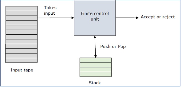
Basic Structure of PDA
A pushdown automaton is a way to implement a context-free grammar in a similar way we design DFA for a regular grammar. A DFA can remember a finite amount of information, but a PDA can remember an infinite amount of information.
Basically a pushdown automaton is −
"Finite state machine" + "a stack"
A pushdown automaton has three components −
- an input tape,
- a control unit, and
- a stack with infinite size.
The stack head scans the top symbol of the stack.
A stack does two operations −
Push − a new symbol is added at the top.
Pop − the top symbol is read and removed.
A PDA may or may not read an input symbol, but it has to read the top of the stack in every transition.
A PDA can be formally described as a 7-tuple (Q, ∑, S, δ, q0, I, F) −
Q is the finite number of states
∑ is input alphabet
S is stack symbols
δ is the transition function: Q × (∑ ∪ {ε}) × S × Q × S*
q0 is the initial state (q0 ∈ Q)
I is the initial stack top symbol (I ∈ S)
F is a set of accepting states (F ∈ Q)
The following diagram shows a transition in a PDA from a state q1 to state q2, labeled as a,b → c −
This means at state q1, if we encounter an input string ‘a’ and top symbol of the stack is ‘b’, then we pop ‘b’, push ‘c’ on top of the stack and move to state q2.
Terminologies Related to PDA
Instantaneous Description
The instantaneous description (ID) of a PDA is represented by a triplet (q, w, s) where
q is the state
w is unconsumed input
s is the stack contents
Turnstile Notation
The "turnstile" notation is used for connecting pairs of ID's that represent one or many moves of a PDA. The process of transition is denoted by the turnstile symbol "⊢".
Consider a PDA (Q, ∑, S, δ, q0, I, F). A transition can be mathematically represented by the following turnstile notation −
(p, aw, Tβ) ⊢ (q, w, αb)This implies that while taking a transition from state p to state q, the input symbol ‘a’ is consumed, and the top of the stack ‘T’ is replaced by a new string ‘α’.
Note − If we want zero or more moves of a PDA, we have to use the symbol (⊢*) for it.
There are two different ways to define PDA acceptability.
Final State Acceptability
In final state acceptability, a PDA accepts a string when, after reading the entire string, the PDA is in a final state. From the starting state, we can make moves that end up in a final state with any stack values. The stack values are irrelevant as long as we end up in a final state.
For a PDA (Q, ∑, S, δ, q0, I, F), the language accepted by the set of final states F is −
L(PDA) = {w | (q0, w, I) ⊢* (q, ε, x), q ∈ F}
for any input stack string x.
Empty Stack Acceptability
Here a PDA accepts a string when, after reading the entire string, the PDA has emptied its stack.
For a PDA (Q, ∑, S, δ, q0, I, F), the language accepted by the empty stack is −
L(PDA) = {w | (q0, w, I) ⊢* (q, ε, ε), q ∈ Q}
Example
Construct a PDA that accepts L = {0n 1n | n ≥ 0}
Solution

This language accepts L = {ε, 01, 0011, 000111, ............................. }
Here, in this example, the number of ‘a’ and ‘b’ have to be same.
Initially we put a special symbol ‘$’ into the empty stack.
Then at state q2, if we encounter input 0 and top is Null, we push 0 into stack. This may iterate. And if we encounter input 1 and top is 0, we pop this 0.
Then at state q3, if we encounter input 1 and top is 0, we pop this 0. This may also iterate. And if we encounter input 1 and top is 0, we pop the top element.
If the special symbol ‘$’ is encountered at top of the stack, it is popped out and it finally goes to the accepting state q4.
Example
Construct a PDA that accepts L = { wwR | w = (a+b)* }
Solution

Initially we put a special symbol ‘$’ into the empty stack. At state q2, the w is being read. In state q3, each 0 or 1 is popped when it matches the input. If any other input is given, the PDA will go to a dead state. When we reach that special symbol ‘$’, we go to the accepting state q4.
If a grammar G is context-free, we can build an equivalent nondeterministic PDA which accepts the language that is produced by the context-free grammar G. A parser can be built for the grammar G.
Also, if P is a pushdown automaton, an equivalent context-free grammar G can be constructed where
L(G) = L(P)
In the next two topics, we will discuss how to convert from PDA to CFG and vice versa.
Algorithm to find PDA corresponding to a given CFG
Input − A CFG, G = (V, T, P, S)
Output − Equivalent PDA, P = (Q, ∑, S, δ, q0, I, F)
Step 1 − Convert the productions of the CFG into GNF.
Step 2 − The PDA will have only one state {q}.
Step 3 − The start symbol of CFG will be the start symbol in the PDA.
Step 4 − All non-terminals of the CFG will be the stack symbols of the PDA and all the terminals of the CFG will be the input symbols of the PDA.
Step 5 − For each production in the form A → aX where a is terminal and A, X are combination of terminal and non-terminals, make a transition δ (q, a, A).
Problem
Construct a PDA from the following CFG.
G = ({S, X}, {a, b}, P, S)
where the productions are −
S → XS | ε , A → aXb | Ab | ab
Solution
Let the equivalent PDA,
P = ({q}, {a, b}, {a, b, X, S}, δ, q, S)
where δ −
δ(q, ε , S) = {(q, XS), (q, ε )}
δ(q, ε , X) = {(q, aXb), (q, Xb), (q, ab)}
δ(q, a, a) = {(q, ε )}
δ(q, 1, 1) = {(q, ε )}
Algorithm to find CFG corresponding to a given PDA
Input − A CFG, G = (V, T, P, S)
Output − Equivalent PDA, P = (Q, ∑, S, δ, q0, I, F) such that the non- terminals of the grammar G will be {Xwx | w,x ∈ Q} and the start state will be Aq0,F.
Step 1 − For every w, x, y, z ∈ Q, m ∈ S and a, b ∈ ∑, if δ (w, a, ε) contains (y, m) and (z, b, m) contains (x, ε), add the production rule Xwx → a Xyzb in grammar G.
Step 2 − For every w, x, y, z ∈ Q, add the production rule Xwx → XwyXyx in grammar G.
Step 3 − For w ∈ Q, add the production rule Xww → ε in grammar G.
Parsing is used to derive a string using the production rules of a grammar. It is used to check the acceptability of a string. Compiler is used to check whether or not a string is syntactically correct. A parser takes the inputs and builds a parse tree.
A parser can be of two types −
Top-Down Parser − Top-down parsing starts from the top with the start-symbol and derives a string using a parse tree.
Bottom-Up Parser − Bottom-up parsing starts from the bottom with the string and comes to the start symbol using a parse tree.
Design of Top-Down Parser
For top-down parsing, a PDA has the following four types of transitions −
Pop the non-terminal on the left hand side of the production at the top of the stack and push its right-hand side string.
If the top symbol of the stack matches with the input symbol being read, pop it.
Push the start symbol ‘S’ into the stack.
If the input string is fully read and the stack is empty, go to the final state ‘F’.
Example
Design a top-down parser for the expression "x+y*z" for the grammar G with the following production rules −
P: S → S+X | X, X → X*Y | Y, Y → (S) | id
Solution
If the PDA is (Q, ∑, S, δ, q0, I, F), then the top-down parsing is −
(x+y*z, I) ⊢(x +y*z, SI) ⊢ (x+y*z, S+XI) ⊢(x+y*z, X+XI)
⊢(x+y*z, Y+X I) ⊢(x+y*z, x+XI) ⊢(+y*z, +XI) ⊢ (y*z, XI)
⊢(y*z, X*YI) ⊢(y*z, y*YI) ⊢(*z,*YI) ⊢(z, YI) ⊢(z, zI) ⊢(ε, I)
Design of a Bottom-Up Parser
For bottom-up parsing, a PDA has the following four types of transitions −
Push the current input symbol into the stack.
Replace the right-hand side of a production at the top of the stack with its left-hand side.
If the top of the stack element matches with the current input symbol, pop it.
If the input string is fully read and only if the start symbol ‘S’ remains in the stack, pop it and go to the final state ‘F’.
Example
Design a top-down parser for the expression "x+y*z" for the grammar G with the following production rules −
P: S → S+X | X, X → X*Y | Y, Y → (S) | id
Solution
If the PDA is (Q, ∑, S, δ, q0, I, F), then the bottom-up parsing is −
(x+y*z, I) ⊢ (+y*z, xI) ⊢ (+y*z, YI) ⊢ (+y*z, XI) ⊢ (+y*z, SI)
⊢(y*z, +SI) ⊢ (*z, y+SI) ⊢ (*z, Y+SI) ⊢ (*z, X+SI) ⊢ (z, *X+SI)
⊢ (ε, z*X+SI) ⊢ (ε, Y*X+SI) ⊢ (ε, X+SI) ⊢ (ε, SI)
A Turing Machine is an accepting device which accepts the languages (recursively enumerable set) generated by type 0 grammars. It was invented in 1936 by Alan Turing.
Definition
A Turing Machine (TM) is a mathematical model which consists of an infinite length tape divided into cells on which input is given. It consists of a head which reads the input tape. A state register stores the state of the Turing machine. After reading an input symbol, it is replaced with another symbol, its internal state is changed, and it moves from one cell to the right or left. If the TM reaches the final state, the input string is accepted, otherwise rejected.
A TM can be formally described as a 7-tuple (Q, X, ∑, δ, q0, B, F) where −
Q is a finite set of states
X is the tape alphabet
∑ is the input alphabet
δ is a transition function; δ : Q × X → Q × X × {Left_shift, Right_shift}.
q0 is the initial state
B is the blank symbol
F is the set of final states
Comparison with the previous automaton
The following table shows a comparison of how a Turing machine differs from Finite Automaton and Pushdown Automaton.
| Machine | Stack Data Structure | Deterministic? |
|---|---|---|
| Finite Automaton | N.A | Yes |
| Pushdown Automaton | Last In First Out(LIFO) | No |
| Turing Machine | Infinite tape | Yes |
Example of Turing machine
Turing machine M = (Q, X, ∑, δ, q0, B, F) with
- Q = {q0, q1, q2, qf}
- X = {a, b}
- ∑ = {1}
- q0 = {q0}
- B = blank symbol
- F = {qf }
δ is given by −
| Tape alphabet symbol | Present State ‘q0’ | Present State ‘q1’ | Present State ‘q2’ |
|---|---|---|---|
| a | 1Rq1 | 1Lq0 | 1Lqf |
| b | 1Lq2 | 1Rq1 | 1Rqf |
Here the transition 1Rq1 implies that the write symbol is 1, the tape moves right, and the next state is q1. Similarly, the transition 1Lq2 implies that the write symbol is 1, the tape moves left, and the next state is q2.
Time and Space Complexity of a Turing Machine
For a Turing machine, the time complexity refers to the measure of the number of times the tape moves when the machine is initialized for some input symbols and the space complexity is the number of cells of the tape written.
Time complexity all reasonable functions −
T(n) = O(n log n)
TM's space complexity −
S(n) = O(n)
A TM accepts a language if it enters into a final state for any input string w. A language is recursively enumerable (generated by Type-0 grammar) if it is accepted by a Turing machine.
A TM decides a language if it accepts it and enters into a rejecting state for any input not in the language. A language is recursive if it is decided by a Turing machine.
There may be some cases where a TM does not stop. Such TM accepts the language, but it does not decide it.
Designing a Turing Machine
The basic guidelines of designing a Turing machine have been explained below with the help of a couple of examples.
Example 1
Design a TM to recognize all strings consisting of an odd number of α’s.
Solution
The Turing machine M can be constructed by the following moves −
Let q1 be the initial state.
If M is in q1; on scanning α, it enters the state q2 and writes B (blank).
If M is in q2; on scanning α, it enters the state q1 and writes B (blank).
From the above moves, we can see that M enters the state q1 if it scans an even number of α’s, and it enters the state q2 if it scans an odd number of α’s. Hence q2 is the only accepting state.
Hence,
M = {{q1, q2}, {1}, {1, B}, δ, q1, B, {q2}}
where δ is given by −
| Tape alphabet symbol | Present State ‘q1’ | Present State ‘q2’ |
|---|---|---|
| α | BRq2 | BRq1 |
Example 2
Design a Turing Machine that reads a string representing a binary number and erases all leading 0’s in the string. However, if the string comprises of only 0’s, it keeps one 0.
Solution
Let us assume that the input string is terminated by a blank symbol, B, at each end of the string.
The Turing Machine, M, can be constructed by the following moves −
Let q0 be the initial state.
If M is in q0, on reading 0, it moves right, enters the state q1 and erases 0. On reading 1, it enters the state q2 and moves right.
If M is in q1, on reading 0, it moves right and erases 0, i.e., it replaces 0’s by B’s. On reaching the leftmost 1, it enters q2 and moves right. If it reaches B, i.e., the string comprises of only 0’s, it moves left and enters the state q3.
If M is in q2, on reading either 0 or 1, it moves right. On reaching B, it moves left and enters the state q4. This validates that the string comprises only of 0’s and 1’s.
If M is in q3, it replaces B by 0, moves left and reaches the final state qf.
If M is in q4, on reading either 0 or 1, it moves left. On reaching the beginning of the string, i.e., when it reads B, it reaches the final state qf.
Hence,
M = {{q0, q1, q2, q3, q4, qf}, {0,1, B}, {1, B}, δ, q0, B, {qf}}
where δ is given by −
| Tape alphabet symbol | Present State ‘q0’ | Present State ‘q1’ | Present State ‘q2’ | Present State ‘q3’ | Present State ‘q4’ |
|---|---|---|---|---|---|
| 0 | BRq1 | BRq1 | ORq2 | - | OLq4 |
| 1 | 1Rq2 | 1Rq2 | 1Rq2 | - | 1Lq4 |
| B | BRq1 | BLq3 | BLq4 | OLqf | BRqf |
Multi-tape Turing Machines have multiple tapes where each tape is accessed with a separate head. Each head can move independently of the other heads. Initially the input is on tape 1 and others are blank. At first, the first tape is occupied by the input and the other tapes are kept blank. Next, the machine reads consecutive symbols under its heads and the TM prints a symbol on each tape and moves its heads.

A Multi-tape Turing machine can be formally described as a 6-tuple (Q, X, B, δ, q0, F) where −
Q is a finite set of states
X is the tape alphabet
B is the blank symbol
δ is a relation on states and symbols where
δ: Q × Xk → Q × (X × {Left_shift, Right_shift, No_shift })k
where there is k number of tapes
q0 is the initial state
F is the set of final states
Note − Every Multi-tape Turing machine has an equivalent single-tape Turing machine.
Multi-track Turing machines, a specific type of Multi-tape Turing machine, contain multiple tracks but just one tape head reads and writes on all tracks. Here, a single tape head reads n symbols from n tracks at one step. It accepts recursively enumerable languages like a normal single-track single-tape Turing Machine accepts.
A Multi-track Turing machine can be formally described as a 6-tuple (Q, X, ∑, δ, q0, F) where −
Q is a finite set of states
X is the tape alphabet
∑ is the input alphabet
δ is a relation on states and symbols where
δ(Qi, [a1, a2, a3,....]) = (Qj, [b1, b2, b3,....], Left_shift or Right_shift)
q0 is the initial state
F is the set of final states
Note − For every single-track Turing Machine S, there is an equivalent multi-track Turing Machine M such that L(S) = L(M).
In a Non-Deterministic Turing Machine, for every state and symbol, there are a group of actions the TM can have. So, here the transitions are not deterministic. The computation of a non-deterministic Turing Machine is a tree of configurations that can be reached from the start configuration.
An input is accepted if there is at least one node of the tree which is an accept configuration, otherwise it is not accepted. If all branches of the computational tree halt on all inputs, the non-deterministic Turing Machine is called a Decider and if for some input, all branches are rejected, the input is also rejected.
A non-deterministic Turing machine can be formally defined as a 6-tuple (Q, X, ∑, δ, q0, B, F) where −
Q is a finite set of states
X is the tape alphabet
∑ is the input alphabet
δ is a transition function;
δ : Q × X → P(Q × X × {Left_shift, Right_shift}).
q0 is the initial state
B is the blank symbol
F is the set of final states
A Turing Machine with a semi-infinite tape has a left end but no right end. The left end is limited with an end marker.

It is a two-track tape −
Upper track − It represents the cells to the right of the initial head position.
Lower track − It represents the cells to the left of the initial head position in reverse order.
The infinite length input string is initially written on the tape in contiguous tape cells.
The machine starts from the initial state q0 and the head scans from the left end marker ‘End’. In each step, it reads the symbol on the tape under its head. It writes a new symbol on that tape cell and then it moves the head either into left or right one tape cell. A transition function determines the actions to be taken.
It has two special states called accept state and reject state. If at any point of time it enters into the accepted state, the input is accepted and if it enters into the reject state, the input is rejected by the TM. In some cases, it continues to run infinitely without being accepted or rejected for some certain input symbols.
Note − Turing machines with semi-infinite tape are equivalent to standard Turing machines.
A linear bounded automaton is a multi-track non-deterministic Turing machine with a tape of some bounded finite length.
Length = function (Length of the initial input string, constant c)
Here,
Memory information ≤ c × Input information
The computation is restricted to the constant bounded area. The input alphabet contains two special symbols which serve as left end markers and right end markers which mean the transitions neither move to the left of the left end marker nor to the right of the right end marker of the tape.
A linear bounded automaton can be defined as an 8-tuple (Q, X, ∑, q0, ML, MR, δ, F) where −
Q is a finite set of states
X is the tape alphabet
∑ is the input alphabet
q0 is the initial state
ML is the left end marker
MR is the right end marker where MR ≠ ML
δ is a transition function which maps each pair (state, tape symbol) to (state, tape symbol, Constant ‘c’) where c can be 0 or +1 or -1
F is the set of final states

A deterministic linear bounded automaton is always context-sensitive and the linear bounded automaton with empty language is undecidable..
A language is called Decidable or Recursive if there is a Turing machine which accepts and halts on every input string w. Every decidable language is Turing-Acceptable.

A decision problem P is decidable if the language L of all yes instances to P is decidable.
For a decidable language, for each input string, the TM halts either at the accept or the reject state as depicted in the following diagram −

Example 1
Find out whether the following problem is decidable or not −
Is a number ‘m’ prime?
Solution
Prime numbers = {2, 3, 5, 7, 11, 13, …………..}
Divide the number ‘m’ by all the numbers between ‘2’ and ‘√m’ starting from ‘2’.
If any of these numbers produce a remainder zero, then it goes to the “Rejected state”, otherwise it goes to the “Accepted state”. So, here the answer could be made by ‘Yes’ or ‘No’.
Hence, it is a decidable problem.
Example 2
Given a regular language L and string w, how can we check if w ∈ L?
Solution
Take the DFA that accepts L and check if w is accepted

Some more decidable problems are −
- Does DFA accept the empty language?
- Is L1 ∩ L2 = ∅ for regular sets?
Note −
If a language L is decidable, then its complement L' is also decidable
If a language is decidable, then there is an enumerator for it.
For an undecidable language, there is no Turing Machine which accepts the language and makes a decision for every input string w (TM can make decision for some input string though). A decision problem P is called “undecidable” if the language L of all yes instances to P is not decidable. Undecidable languages are not recursive languages, but sometimes, they may be recursively enumerable languages.

Example
- The halting problem of Turing machine
- The mortality problem
- The mortal matrix problem
- The Post correspondence problem, etc.
Input − A Turing machine and an input string w.
Problem − Does the Turing machine finish computing of the string w in a finite number of steps? The answer must be either yes or no.
Proof − At first, we will assume that such a Turing machine exists to solve this problem and then we will show it is contradicting itself. We will call this Turing machine as a Halting machine that produces a ‘yes’ or ‘no’ in a finite amount of time. If the halting machine finishes in a finite amount of time, the output comes as ‘yes’, otherwise as ‘no’. The following is the block diagram of a Halting machine −

Now we will design an inverted halting machine (HM)’ as −
If H returns YES, then loop forever.
If H returns NO, then halt.
The following is the block diagram of an ‘Inverted halting machine’ −

Further, a machine (HM)2 which input itself is constructed as follows −
- If (HM)2 halts on input, loop forever.
- Else, halt.
Here, we have got a contradiction. Hence, the halting problem is undecidable.
Rice theorem states that any non-trivial semantic property of a language which is recognized by a Turing machine is undecidable. A property, P, is the language of all Turing machines that satisfy that property.
Formal Definition
If P is a non-trivial property, and the language holding the property, Lp , is recognized by Turing machine M, then Lp = {<M> | L(M) ∈ P} is undecidable.
Description and Properties
Property of languages, P, is simply a set of languages. If any language belongs to P (L ∈ P), it is said that L satisfies the property P.
A property is called to be trivial if either it is not satisfied by any recursively enumerable languages, or if it is satisfied by all recursively enumerable languages.
A non-trivial property is satisfied by some recursively enumerable languages and are not satisfied by others. Formally speaking, in a non-trivial property, where L ∈ P, both the following properties hold:
Property 1 − There exists Turing Machines, M1 and M2 that recognize the same language, i.e. either ( <M1>, <M2> ∈ L ) or ( <M1>,<M2> ∉ L )
Property 2 − There exists Turing Machines M1 and M2, where M1 recognizes the language while M2 does not, i.e. <M1> ∈ L and <M2> ∉ L
Proof
Suppose, a property P is non-trivial and φ ∈ P.
Since, P is non-trivial, at least one language satisfies P, i.e., L(M0) ∈ P , ∋ Turing Machine M0.
Let, w be an input in a particular instant and N is a Turing Machine which follows −
On input x
- Run M on w
- If M does not accept (or doesn't halt), then do not accept x (or do not halt)
- If M accepts w then run M0 on x. If M0 accepts x, then accept x.
A function that maps an instance ATM = {<M,w>| M accepts input w} to a N such that
- If M accepts w and N accepts the same language as M0, Then L(M) = L(M0) ∈ p
- If M does not accept w and N accepts φ, Then L(N) = φ ∉ p
Since ATM is undecidable and it can be reduced to Lp, Lp is also undecidable.
The Post Correspondence Problem (PCP), introduced by Emil Post in 1946, is an undecidable decision problem. The PCP problem over an alphabet ∑ is stated as follows −
Given the following two lists, M and N of non-empty strings over ∑ −
M = (x1, x2, x3,………, xn)
N = (y1, y2, y3,………, yn)
We can say that there is a Post Correspondence Solution, if for some i1,i2,………… ik, where 1 ≤ ij ≤ n, the condition xi1 …….xik = yi1 …….yik satisfies.
Example 1
Find whether the lists
M = (abb, aa, aaa) and N = (bba, aaa, aa)
have a Post Correspondence Solution?
Solution
| x1 | x2 | x3 | |
|---|---|---|---|
| M | Abb | aa | aaa |
| N | Bba | aaa | aa |
Here,
x2x1x3 = ‘aaabbaaa’
and y2y1y3 = ‘aaabbaaa’
We can see that
x2x1x3 = y2y1y3
Hence, the solution is i = 2, j = 1, and k = 3.
Example 2
Find whether the lists M = (ab, bab, bbaaa) and N = (a, ba, bab) have a Post Correspondence Solution?
Solution
| x1 | x2 | x3 | |
|---|---|---|---|
| M | ab | bab | bbaaa |
| N | a | ba | bab |
In this case, there is no solution because −
| x2x1x3 | ≠ | y2y1y3 | (Lengths are not same)
Hence, it can be said that this Post Correspondence Problem is undecidable.