Teoria degli automi - Guida rapida
Automi: che cos'è?
Il termine "automi" deriva dalla parola greca "αὐτόματα" che significa "auto-agente". Un automa (Automata al plurale) è un dispositivo informatico semovente astratto che segue automaticamente una sequenza predeterminata di operazioni.
Un automa con un numero finito di stati è chiamato a Finite Automaton (FA) o Finite State Machine (FSM).
Definizione formale di un automa finito
Un automa può essere rappresentato da una tupla di 5 (Q, ∑, δ, q 0 , F), dove -
Q è un insieme finito di stati.
∑ è un insieme finito di simboli, chiamato alphabet dell'automa.
δ è la funzione di transizione.
q0è lo stato iniziale da cui viene elaborato qualsiasi input (q 0 ∈ Q).
F è un insieme di stati finali di Q (F ⊆ Q).
Terminologie correlate
Alfabeto
Definition - An alphabet è un insieme finito di simboli.
Example - ∑ = {a, b, c, d} è un alphabet set dove sono "a", "b", "c" e "d" symbols.
Corda
Definition - A string è una sequenza finita di simboli presi da ∑.
Example - 'cabcad' è una stringa valida nel set alfabetico ∑ = {a, b, c, d}
Lunghezza di una stringa
Definition- È il numero di simboli presenti in una stringa. (Denotato da|S|).
Examples -
Se S = 'cabcad', | S | = 6
Se | S | = 0, viene chiamato un empty string (Denotato da λ o ε)
Kleene Star
Definition - La star di Kleene, ∑*, è un operatore unario su un insieme di simboli o stringhe, ∑, che fornisce l'insieme infinito di tutte le possibili stringhe di tutte le lunghezze possibili ∑ Compreso λ.
Representation- ∑ * = ∑ 0 ∪ ∑ 1 ∪ ∑ 2 ∪ ……. dove ∑ p è l'insieme di tutte le possibili stringhe di lunghezza p.
Example - Se ∑ = {a, b}, ∑ * = {λ, a, b, aa, ab, ba, bb, ……… ..}
Chiusura Kleene / Plus
Definition - Il set ∑+ è l'insieme infinito di tutte le possibili stringhe di tutte le lunghezze possibili su ∑ escluso λ.
Representation- ∑ + = ∑ 1 ∪ ∑ 2 ∪ ∑ 3 ∪ …….
∑ + = ∑ * - {λ}
Example- Se ∑ = {a, b}, ∑ + = {a, b, aa, ab, ba, bb, ……… ..}
linguaggio
Definition- Una lingua è un sottoinsieme di ∑ * per alcuni alfabeti ∑. Può essere finito o infinito.
Example - Se la lingua accetta tutte le possibili stringhe di lunghezza 2 su ∑ = {a, b}, allora L = {ab, aa, ba, bb}
Finite Automaton può essere classificato in due tipi:
- Automa finito deterministico (DFA)
- Automa finito non deterministico (NDFA / NFA)
Automa finito deterministico (DFA)
In DFA, per ogni simbolo di input, è possibile determinare lo stato in cui si sposterà la macchina. Quindi, si chiamaDeterministic Automaton. Poiché ha un numero finito di stati, la macchina viene chiamataDeterministic Finite Machine o Deterministic Finite Automaton.
Definizione formale di un DFA
Un DFA può essere rappresentato da una tupla di 5 (Q, ∑, δ, q 0 , F) dove -
Q è un insieme finito di stati.
∑ è un insieme finito di simboli chiamato alfabeto.
δ è la funzione di transizione dove δ: Q × ∑ → Q
q0è lo stato iniziale da cui viene elaborato qualsiasi input (q 0 ∈ Q).
F è un insieme di stati finali di Q (F ⊆ Q).
Rappresentazione grafica di un DFA
Un DFA è rappresentato da digrafi chiamati state diagram.
- I vertici rappresentano gli stati.
- Gli archi etichettati con un alfabeto di input mostrano le transizioni.
- Lo stato iniziale è indicato da un singolo arco in entrata vuoto.
- Lo stato finale è indicato da doppi cerchi.
Esempio
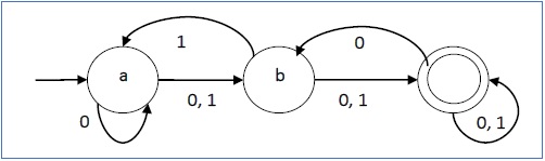
Sia un automa finito deterministico →
- Q = {a, b, c},
- ∑ = {0, 1},
- q 0 = {a},
- F = {c} e
Funzione di transizione δ come mostrato dalla tabella seguente -
| Stato attuale | Stato successivo per ingresso 0 | Stato successivo per ingresso 1 |
|---|---|---|
| a | un | b |
| b | c | un |
| c | b | c |
La sua rappresentazione grafica sarebbe la seguente:

In NDFA, per un particolare simbolo di input, la macchina può spostarsi in qualsiasi combinazione degli stati nella macchina. In altre parole, non è possibile determinare lo stato esatto in cui si muove la macchina. Quindi, si chiamaNon-deterministic Automaton. Poiché ha un numero finito di stati, la macchina viene chiamataNon-deterministic Finite Machine o Non-deterministic Finite Automaton.
Definizione formale di un NDFA
Un NDFA può essere rappresentato da una tupla di 5 (Q, ∑, δ, q 0 , F) dove -
Q è un insieme finito di stati.
∑ è un insieme finito di simboli chiamati alfabeti.
δè la funzione di transizione dove δ: Q × ∑ → 2 Q
(Qui è stato preso il set di potenza di Q (2 Q ) perché in caso di NDFA, da uno stato, la transizione può avvenire a qualsiasi combinazione di stati Q)
q0è lo stato iniziale da cui viene elaborato qualsiasi input (q 0 ∈ Q).
F è un insieme di stati finali di Q (F ⊆ Q).
Rappresentazione grafica di un NDFA: (uguale a DFA)
Un NDFA è rappresentato da digrafi chiamati diagramma di stato.
- I vertici rappresentano gli stati.
- Gli archi etichettati con un alfabeto di input mostrano le transizioni.
- Lo stato iniziale è indicato da un singolo arco in entrata vuoto.
- Lo stato finale è indicato da doppi cerchi.
Example
Sia un automa finito non deterministico →
- Q = {a, b, c}
- ∑ = {0, 1}
- q 0 = {a}
- F = {c}
La funzione di transizione δ come mostrato di seguito -
| Stato attuale | Stato successivo per ingresso 0 | Stato successivo per ingresso 1 |
|---|---|---|
| un | a, b | b |
| b | c | corrente alternata |
| c | avanti Cristo | c |
La sua rappresentazione grafica sarebbe la seguente:
DFA vs NDFA
La tabella seguente elenca le differenze tra DFA e NDFA.
| DFA | NDFA |
|---|---|
| La transizione da uno stato è a un singolo particolare stato successivo per ogni simbolo di ingresso. Quindi è chiamato deterministico . | La transizione da uno stato può avvenire a più stati successivi per ogni simbolo di ingresso. Quindi è chiamato non deterministico . |
| Le transizioni di stringhe vuote non vengono visualizzate in DFA. | NDFA consente transizioni di stringhe vuote. |
| Il backtracking è consentito in DFA | In NDFA, il backtracking non è sempre possibile. |
| Richiede più spazio. | Richiede meno spazio. |
| Una stringa viene accettata da un DFA, se transita in uno stato finale. | Una stringa viene accettata da un NDFA, se almeno una di tutte le possibili transizioni termina in uno stato finale. |
Accettori, classificatori e trasduttori
Accettatore (Riconoscitore)
Un automa che calcola una funzione booleana è chiamato un acceptor. Tutti gli stati di un accettore accettano o rifiutano gli input forniti.
Classificatore
UN classifier ha più di due stati finali e fornisce un singolo output quando termina.
Trasduttore
Un automa che produce output in base all'input corrente e / o allo stato precedente è chiamato a transducer. I trasduttori possono essere di due tipi:
Mealy Machine - L'uscita dipende sia dallo stato corrente che dall'ingresso corrente.
Moore Machine - L'uscita dipende solo dallo stato corrente.
Accettabilità da parte di DFA e NDFA
Una stringa viene accettata da un DFA / NDFA se e solo se il DFA / NDFA che inizia dallo stato iniziale finisce in uno stato di accettazione (uno degli stati finali) dopo aver letto interamente la stringa.
Una stringa S è accettata da un DFA / NDFA (Q, ∑, δ, q 0 , F), iff
δ*(q0, S) ∈ F
La lingua L accettato da DFA / NDFA è
{S | S ∈ ∑* and δ*(q0, S) ∈ F}
Una stringa S ′ non è accettata da un DFA / NDFA (Q, ∑, δ, q 0 , F), se e solo
δ*(q0, S′) ∉ F
La lingua L ′ non accettata da DFA / NDFA (Complemento della lingua accettata L) è
{S | S ∈ ∑* and δ*(q0, S) ∉ F}
Example
Consideriamo il DFA mostrato nella Figura 1.3. Da DFA è possibile derivare le stringhe accettabili.

Stringhe accettate dal DFA precedente: {0, 00, 11, 010, 101, ...........}
Stringhe non accettate dal DFA precedente: {1, 011, 111, ........}
Dichiarazione problema
Permettere X = (Qx, ∑, δx, q0, Fx)essere un NDFA che accetta il linguaggio L (X). Dobbiamo progettare un DFA equivalenteY = (Qy, ∑, δy, q0, Fy) tale che L(Y) = L(X). La procedura seguente converte l'NDFA nel suo DFA equivalente:
Algoritmo
Input - Un NDFA
Output - Un DFA equivalente
Step 1 - Crea una tabella di stato dal dato NDFA.
Step 2 - Creare una tabella di stato vuota sotto i possibili alfabeti di input per il DFA equivalente.
Step 3 - Contrassegna lo stato iniziale del DFA con q0 (uguale all'NDFA).
Step 4- Trova la combinazione di Stati {Q 0 , Q 1 , ..., Q n } per ogni possibile alfabeto di input.
Step 5 - Ogni volta che generiamo un nuovo stato DFA sotto le colonne alfabetiche di input, dobbiamo applicare nuovamente il passaggio 4, altrimenti andare al passaggio 6.
Step 6 - Gli stati che contengono uno degli stati finali dell'NDFA sono gli stati finali dell'equivalente DFA.
Esempio
Consideriamo l'NDFA mostrato nella figura seguente.

| q | δ (q, 0) | δ (q, 1) |
|---|---|---|
| un | {a, b, c, d, e} | {d, e} |
| b | {c} | {e} |
| c | ∅ | {b} |
| d | {e} | ∅ |
| e | ∅ | ∅ |
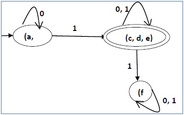
Utilizzando l'algoritmo di cui sopra, troviamo il suo equivalente DFA. La tabella degli stati di DFA è mostrata di seguito.
| q | δ (q, 0) | δ (q, 1) |
|---|---|---|
| [un] | [a, b, c, d, e] | [d, e] |
| [a, b, c, d, e] | [a, b, c, d, e] | [b, d, e] |
| [d, e] | [e] | ∅ |
| [b, d, e] | [c, e] | [e] |
| [e] | ∅ | ∅ |
| [c, e] | ∅ | [b] |
| [b] | [c] | [e] |
| [c] | ∅ | [b] |
Il diagramma di stato del DFA è il seguente:

Minimizzazione di DFA utilizzando il teorema di Myhill-Nerode
Algoritmo
Input - DFA
Output - DFA ridotto a icona
Step 1- Disegna una tabella per tutte le coppie di stati (Q i , Q j ) non necessariamente collegati direttamente [Tutti sono inizialmente non contrassegnati]
Step 2- Considera ogni coppia di stati (Q i , Q j ) nel DFA dove Q i ∈ F e Q j ∉ F o viceversa e contrassegnale. [Qui F è l'insieme degli stati finali]
Step 3 - Ripeti questo passaggio fino a quando non sarà più possibile contrassegnare gli stati -
Se è presente una coppia non contrassegnata (Q i , Q j ), contrassegnala se la coppia {δ (Q i , A), δ (Q i , A)} è contrassegnata per qualche alfabeto di input.
Step 4- Combina tutte le coppie non contrassegnate (Q i , Q j ) e trasformale in un unico stato nel DFA ridotto.
Esempio
Utilizziamo l'algoritmo 2 per ridurre al minimo il DFA mostrato di seguito.

Step 1 - Disegniamo una tabella per tutte le coppie di stati.
| un | b | c | d | e | f | |
| un | ||||||
| b | ||||||
| c | ||||||
| d | ||||||
| e | ||||||
| f |
Step 2 - Contrassegniamo le coppie di stato.
| un | b | c | d | e | f | |
| un | ||||||
| b | ||||||
| c | ✔ | ✔ | ||||
| d | ✔ | ✔ | ||||
| e | ✔ | ✔ | ||||
| f | ✔ | ✔ | ✔ |
Step 3- Cercheremo di contrassegnare le coppie di stato, con segno di spunta di colore verde, in modo transitorio. Se inseriamo 1 per indicare "a" e "f", andrà rispettivamente nello stato "c" e "f". (c, f) è già contrassegnato, quindi contrassegneremo la coppia (a, f). Ora, inseriamo 1 per indicare "b" e "f"; andrà rispettivamente nello stato "d" e "f". (d, f) è già contrassegnato, quindi contrassegneremo la coppia (b, f).
| un | b | c | d | e | f | |
| un | ||||||
| b | ||||||
| c | ✔ | ✔ | ||||
| d | ✔ | ✔ | ||||
| e | ✔ | ✔ | ||||
| f | ✔ | ✔ | ✔ | ✔ | ✔ |
Dopo il passaggio 3, abbiamo combinazioni di stati {a, b} {c, d} {c, e} {d, e} che non sono contrassegnate.
Possiamo ricombinare {c, d} {c, e} {d, e} in {c, d, e}
Quindi abbiamo due stati combinati come - {a, b} e {c, d, e}
Quindi il DFA finale ridotto a icona conterrà tre stati {f}, {a, b} e {c, d, e}
Minimizzazione di DFA utilizzando il teorema di equivalenza
Se X e Y sono due stati in un DFA, possiamo combinare questi due stati in {X, Y} se non sono distinguibili. Due stati sono distinguibili, se c'è almeno una stringa S, tale che uno tra δ (X, S) e δ (Y, S) sia accettabile e un altro non accettante. Quindi, un DFA è minimo se e solo se tutti gli stati sono distinguibili.
Algoritmo 3
Step 1 - Tutti gli stati Q sono divisi in due partizioni - final states e non-final states e sono indicati da P0. Tutti gli stati in una partizione sono 0 ° equivalente. Prendi un contatorek e inizializzalo con 0.
Step 2- Incrementa k di 1. Per ogni partizione in P k , dividi gli stati in P k in due partizioni se sono k-distinguibili. Due stati all'interno di questa partizione X e Y sono k-distinguibili se c'è un inputS tale che δ(X, S) e δ(Y, S) sono (k-1) -distinguibili.
Step 3- Se P k ≠ P k-1 , ripetere il passaggio 2, altrimenti andare al passaggio 4.
Step 4- Combina i k- esimi insiemi equivalenti e rendili i nuovi stati del DFA ridotto.
Esempio
Consideriamo il seguente DFA:

| q | δ (q, 0) | δ (q, 1) |
|---|---|---|
| un | b | c |
| b | un | d |
| c | e | f |
| d | e | f |
| e | e | f |
| f | f | f |
Applichiamo l'algoritmo di cui sopra al suddetto DFA -
- P 0 = {(c, d, e), (a, b, f)}
- P 1 = {(c, d, e), (a, b), (f)}
- P 2 = {(c, d, e), (a, b), (f)}
Quindi, P 1 = P 2 .
Ci sono tre stati nel DFA ridotto. Il DFA ridotto è il seguente:
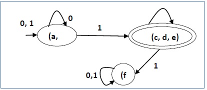
| Q | δ (q, 0) | δ (q, 1) |
|---|---|---|
| (a, b) | (a, b) | (c, d, e) |
| (c, d, e) | (c, d, e) | (f) |
| (f) | (f) | (f) |
Gli automi finiti possono avere uscite corrispondenti a ciascuna transizione. Esistono due tipi di macchine a stati finiti che generano output:
- Macchina farinosa
- Macchina di Moore
Macchina farinosa
Una Mealy Machine è una FSM il cui output dipende dallo stato attuale e dall'input presente.
Può essere descritto da una tupla 6 (Q, ∑, O, δ, X, q 0 ) dove -
Q è un insieme finito di stati.
∑ è un insieme finito di simboli chiamato alfabeto di input.
O è un insieme finito di simboli chiamato alfabeto di output.
δ è la funzione di transizione di ingresso dove δ: Q × ∑ → Q
X è la funzione di transizione dell'uscita dove X: Q × ∑ → O
q0è lo stato iniziale da cui viene elaborato qualsiasi input (q 0 ∈ Q).
La tabella degli stati di una macchina farinosa è mostrata di seguito:
| Stato attuale | Stato successivo | |||
|---|---|---|---|---|
| ingresso = 0 | ingresso = 1 | |||
| Stato | Produzione | Stato | Produzione | |
| → a | b | x 1 | c | x 1 |
| b | b | x 2 | d | x 3 |
| c | d | x 3 | c | x 1 |
| d | d | x 3 | d | x 2 |
Il diagramma di stato della suddetta Mealy Machine è:

Moore Machine
La macchina Moore è una FSM i cui output dipendono solo dallo stato presente.
Una macchina di Moore può essere descritta da una tupla 6 (Q, ∑, O, δ, X, q 0 ) dove -
Q è un insieme finito di stati.
∑ è un insieme finito di simboli chiamato alfabeto di input.
O è un insieme finito di simboli chiamato alfabeto di output.
δ è la funzione di transizione di ingresso dove δ: Q × ∑ → Q
X è la funzione di transizione dell'uscita dove X: Q → O
q0è lo stato iniziale da cui viene elaborato qualsiasi input (q 0 ∈ Q).
La tabella degli stati di una macchina Moore è mostrata di seguito:
| Stato attuale | Stato successivo | Produzione | |
|---|---|---|---|
| Ingresso = 0 | Ingresso = 1 | ||
| → a | b | c | x 2 |
| b | b | d | x 1 |
| c | c | d | x 2 |
| d | d | d | x 3 |
Il diagramma di stato della macchina Moore sopra è:

Mealy Machine contro Moore Machine
La tabella seguente evidenzia i punti che differenziano una Mealy Machine da una Moore Machine.
| Macchina farinosa | Moore Machine |
|---|---|
| L'uscita dipende sia dallo stato presente che dall'ingresso presente | L'output dipende solo dallo stato attuale. |
| In generale, ha meno stati di Moore Machine. | In generale, ha più stati di Mealy Machine. |
| Il valore della funzione di uscita è una funzione delle transizioni e dei cambiamenti, quando viene eseguita la logica di ingresso sullo stato attuale. | Il valore della funzione di uscita è una funzione dello stato corrente e dei cambiamenti ai fronti di clock, ogni volta che si verificano cambiamenti di stato. |
| Le macchine farinose reagiscono più velocemente agli input. Generalmente reagiscono nello stesso ciclo di clock. | Nelle macchine Moore, è necessaria più logica per decodificare le uscite, con conseguenti più ritardi del circuito. Generalmente reagiscono dopo un ciclo di clock. |
Moore Machine to Mealy Machine
Algoritmo 4
Input - Moore Machine
Output - Macchina farinosa
Step 1 - Prendi un formato di tabella di transizione Mealy Machine vuoto.
Step 2 - Copia tutti gli stati di transizione della Moore Machine in questo formato di tabella.
Step 3- Verificare gli stati presenti e le relative uscite nella tabella degli stati della macchina Moore; se per uno stato Q i l' output è m, copiarlo nelle colonne di output della tabella di stato Mealy Machine ovunque Q i appare nello stato successivo.
Esempio
Consideriamo la seguente macchina Moore:
| Stato attuale | Stato successivo | Produzione | |
|---|---|---|---|
| a = 0 | a = 1 | ||
| → a | d | b | 1 |
| b | un | d | 0 |
| c | c | c | 0 |
| d | b | un | 1 |
Ora applichiamo l'algoritmo 4 per convertirlo in Mealy Machine.
Step 1 & 2 -
| Stato attuale | Stato successivo | |||
|---|---|---|---|---|
| a = 0 | a = 1 | |||
| Stato | Produzione | Stato | Produzione | |
| → a | d | b | ||
| b | un | d | ||
| c | c | c | ||
| d | b | un | ||
Step 3 -
| Stato attuale | Stato successivo | |||
|---|---|---|---|---|
| a = 0 | a = 1 | |||
| Stato | Produzione | Stato | Produzione | |
| => a | d | 1 | b | 0 |
| b | un | 1 | d | 1 |
| c | c | 0 | c | 0 |
| d | b | 0 | un | 1 |
Mealy Machine to Moore Machine
Algoritmo 5
Input - Macchina farinosa
Output - Moore Machine
Step 1- Calcola il numero di differenti uscite per ogni stato (Q i ) che sono disponibili nella tabella degli stati della macchina Mealy.
Step 2- Se tutte le uscite di Qi sono uguali, copia lo stato Q i . Se ha n uscite distinte, spezza Q i in n stati come Q in doven = 0, 1, 2 .......
Step 3 - Se l'uscita dello stato iniziale è 1, inserire un nuovo stato iniziale all'inizio che restituisce 0 output.
Esempio
Consideriamo la seguente macchina farinosa:
| Stato attuale | Stato successivo | |||
|---|---|---|---|---|
| a = 0 | a = 1 | |||
| Stato successivo | Produzione | Stato successivo | Produzione | |
| → a | d | 0 | b | 1 |
| b | un | 1 | d | 0 |
| c | c | 1 | c | 0 |
| d | b | 0 | un | 1 |
Qui, gli stati "a" e "d" forniscono rispettivamente solo 1 e 0 output, quindi conserviamo gli stati "a" e "d". Ma gli stati "b" e "c" producono output diversi (1 e 0). Quindi, ci dividiamob in b0, b1 e c in c0, c1.
| Stato attuale | Stato successivo | Produzione | |
|---|---|---|---|
| a = 0 | a = 1 | ||
| → a | d | b 1 | 1 |
| b 0 | un | d | 0 |
| b 1 | un | d | 1 |
| c 0 | c 1 | C 0 | 0 |
| c 1 | c 1 | C 0 | 1 |
| d | b 0 | un | 0 |
Nel senso letterario del termine, le grammatiche denotano regole sintattiche per la conversazione nelle lingue naturali. La linguistica ha tentato di definire le grammatiche sin dall'inizio delle lingue naturali come l'inglese, il sanscrito, il mandarino, ecc.
La teoria dei linguaggi formali trova la sua applicabilità ampiamente nei campi dell'informatica. Noam Chomsky ha fornito un modello matematico di grammatica nel 1956 che è efficace per la scrittura di linguaggi informatici.
Grammatica
Una grammatica G può essere formalmente scritto come una tupla di 4 (N, T, S, P) dove -
N o VN è un insieme di variabili o simboli non terminali.
T o ∑ è un insieme di simboli di Terminale.
S è una variabile speciale chiamata simbolo Start, S ∈ N
Pè Regole di produzione per terminali e non terminali. Una regola di produzione ha la forma α → β, dove α e β sono stringhe su V N ∪ Σ e almeno un simbolo di α appartiene V N .
Esempio
Grammatica G1 -
({S, A, B}, {a, b}, S, {S → AB, A → a, B → b})
Qui,
S, A, e B sono simboli non terminali;
a e b sono simboli terminali
S è il simbolo Start, S ∈ N
Produzioni, P : S → AB, A → a, B → b
Esempio
Grammatica G2 -
(({S, A}, {a, b}, S, {S → aAb, aA → aaAb, A → ε})
Qui,
S e A sono simboli non terminali.
a e b sono simboli terminali.
ε è una stringa vuota.
S è il simbolo Start, S ∈ N
Produzione P : S → aAb, aA → aaAb, A → ε
Derivazioni da una grammatica
Le stringhe possono essere derivate da altre stringhe utilizzando le produzioni in una grammatica. Se una grammaticaG ha una produzione α → β, possiamo dirlo x α y deriva x β y in G. Questa derivazione è scritta come -
x α y ⇒G x β y
Esempio
Consideriamo la grammatica -
G2 = ({S, A}, {a, b}, S, {S → aAb, aA → aaAb, A → ε})
Alcune delle stringhe che possono essere derivate sono:
S ⇒ aA b utilizzando la produzione S → aAb
⇒ a aA bb utilizzando la produzione aA → aAb
⇒ aaa A bbb utilizzando la produzione aA → aAb
⇒ aaabbb utilizzando la produzione A → ε
Si dice che l'insieme di tutte le stringhe che possono essere derivate da una grammatica sia il linguaggio generato da quella grammatica. Una lingua generata da una grammaticaG è un sottoinsieme definito formalmente da
L (Sol) = {W | W ∈ ∑ *, S ⇒ G W }
Se L(G1) = L(G2), la grammatica G1 è equivalente alla grammatica G2.
Esempio
Se c'è una grammatica
G: N = {S, A, B} T = {a, b} P = {S → AB, A → a, B → b}
Qui S produce ABe possiamo sostituire A di a, e B di b. Qui, l'unica stringa accettata èab, cioè
L (G) = {ab}
Esempio
Supponiamo di avere la seguente grammatica:
G: N = {S, A, B} T = {a, b} P = {S → AB, A → aA | a, B → bB | b}
La lingua generata da questa grammatica -
L (Sol) = {ab, a 2 b, ab 2 , a 2 b 2 , ………}
= {a m b n | m ≥ 1 en ≥ 1}
Costruzione di una grammatica che genera una lingua
Prenderemo in considerazione alcune lingue e le convertiremo in una grammatica G che produce quelle lingue.
Esempio
Problem- Supponiamo che L (G) = {a m b n | m ≥ 0 e n> 0}. Dobbiamo scoprire la grammaticaG che produce L(G).
Solution
Poiché L (G) = {a m b n | m ≥ 0 e n> 0}
l'insieme di stringhe accettate può essere riscritto come -
L (G) = {b, ab, bb, aab, abb, …….}
Qui, il simbolo di inizio deve prendere almeno una "b" preceduta da un numero qualsiasi di "a" incluso null.
Per accettare l'insieme di stringhe {b, ab, bb, aab, abb, …….}, Abbiamo preso le produzioni -
S → aS, S → B, B → be B → bB
S → B → b (Accettato)
S → B → bB → bb (Accettato)
S → aS → aB → ab (Accettato)
S → aS → aaS → aaB → aab (Accettato)
S → aS → aB → abB → abb (Accettato)
Quindi, possiamo provare che ogni singola stringa in L (G) è accettata dal linguaggio generato dall'insieme di produzione.
Da qui la grammatica -
G: ({S, A, B}, {a, b}, S, {S → aS | B, B → b | bB})
Esempio
Problem- Supponiamo che L (G) = {a m b n | m> 0 e n ≥ 0}. Dobbiamo scoprire la grammatica G che produce L (G).
Solution -
Poiché L (G) = {a m b n | m> 0 en ≥ 0}, l'insieme di stringhe accettate può essere riscritto come -
L (G) = {a, aa, ab, aaa, aab, abb, …….}
Qui, il simbolo di inizio deve prendere almeno una "a" seguita da un numero qualsiasi di "b" incluso null.
Per accettare l'insieme di stringhe {a, aa, ab, aaa, aab, abb, …….}, Abbiamo preso le produzioni -
S → aA, A → aA, A → B, B → bB, B → λ
S → aA → aB → aλ → a (Accettato)
S → aA → aaA → aaB → aaλ → aa (Accettato)
S → aA → aB → abB → abλ → ab (Accettato)
S → aA → aaA → aaaA → aaaB → aaaλ → aaa (Accettato)
S → aA → aaA → aaB → aabB → aabλ → aab (Accettato)
S → aA → aB → abB → abbB → abbλ → abb (Accettato)
Quindi, possiamo provare che ogni singola stringa in L (G) è accettata dal linguaggio generato dall'insieme di produzione.
Da qui la grammatica -
G: ({S, A, B}, {a, b}, S, {S → aA, A → aA | B, B → λ | bB})
Secondo Noam Chomosky, ci sono quattro tipi di grammatiche: Tipo 0, Tipo 1, Tipo 2 e Tipo 3. La tabella seguente mostra come differiscono l'una dall'altra -
| Tipo di grammatica | Grammatica accettata | Lingua accettata | Automa |
|---|---|---|---|
| Digita 0 | Grammatica illimitata | Linguaggio enumerabile ricorsivamente | Macchina di Turing |
| Tipo 1 | Grammatica sensibile al contesto | Linguaggio sensibile al contesto | Automa lineare limitato |
| Tipo 2 | Grammatica senza contesto | Linguaggio senza contesto | Automa a spinta |
| Tipo 3 | Grammatica regolare | Linguaggio regolare | Automa a stati finiti |
Dai un'occhiata alla seguente illustrazione. Mostra l'ambito di ogni tipo di grammatica -

Tipo - 3 grammatica
Type-3 grammarsgenerare linguaggi regolari. Le grammatiche di tipo 3 devono avere un singolo non terminale sul lato sinistro e un lato destro costituito da un singolo terminale o singolo terminale seguito da un singolo non terminale.
Le produzioni devono essere nella forma X → a or X → aY
dove X, Y ∈ N (Non terminale)
e a ∈ T (Terminale)
La regola S → ε è consentito se S non appare a destra di nessuna regola.
Esempio
X → ε
X → a | aY
Y → b
Tipo - 2 grammatica
Type-2 grammars generare linguaggi privi di contesto.
Le produzioni devono essere nella forma A → γ
dove A ∈ N (Non terminale)
e γ ∈ (T ∪ N)* (Stringa di terminali e non terminali).
Questi linguaggi generati da queste grammatiche sono riconosciuti da un automa pushdown non deterministico.
Esempio
S → X a
X → a
X → aX
X → abc
X → ε
Tipo - 1 grammatica
Type-1 grammarsgenerare linguaggi sensibili al contesto. Le produzioni devono essere nella forma
α A β → α γ β
dove A ∈ N (Non terminale)
e α, β, γ ∈ (T ∪ N)* (Stringhe di terminali e non terminali)
Le corde α e β potrebbe essere vuoto, ma γ non deve essere vuoto.
La regola S → εè consentito se S non compare a destra di nessuna regola. I linguaggi generati da queste grammatiche sono riconosciuti da un automa lineare limitato.
Esempio
AB → AbBc
A → bcA
B → b
Tipo - 0 grammatica
Type-0 grammarsgenerare linguaggi enumerabili ricorsivamente. Le produzioni non hanno restrizioni. Sono qualsiasi grammatica a struttura di fase comprese tutte le grammatiche formali.
Generano i linguaggi riconosciuti da una macchina di Turing.
Le produzioni possono essere sotto forma di α → β dove α è una stringa di terminali e non terminali con almeno un non terminale e α non può essere nullo. β è una stringa di terminali e non terminali.
Esempio
S → ACaB
Bc → acB
CB → DB
aD → Db
UN Regular Expression può essere definito ricorsivamente come segue:
ε è un'espressione regolare indica la lingua contenente una stringa vuota. (L (ε) = {ε})
φ è un'espressione regolare che denota una lingua vuota. (L (φ) = { })
x è un'espressione regolare dove L = {x}
Se X è un'espressione regolare che denota la lingua L(X) e Y è un'espressione regolare che denota la lingua L(Y), poi
X + Y è un'espressione regolare corrispondente alla lingua L(X) ∪ L(Y) dove L(X+Y) = L(X) ∪ L(Y).
X . Y è un'espressione regolare corrispondente alla lingua L(X) . L(Y) dove L(X.Y) = L(X) . L(Y)
R* è un'espressione regolare corrispondente alla lingua L(R*)dove L(R*) = (L(R))*
Se applichiamo una delle regole più volte da 1 a 5, si tratta di espressioni regolari.
Alcuni esempi di RE
| Espressioni regolari | Set regolare |
|---|---|
| (0 + 10 *) | L = {0, 1, 10, 100, 1000, 10000,…} |
| (0 * 10 *) | L = {1, 01, 10, 010, 0010,…} |
| (0 + ε) (1 + ε) | L = {ε, 0, 1, 01} |
| (a + b) * | Insieme di stringhe di a e b di qualsiasi lunghezza inclusa la stringa nulla. Quindi L = {ε, a, b, aa, ab, bb, ba, aaa …….} |
| (a + b) * abb | Insieme di stringhe di a e b che terminano con la stringa abb. Quindi L = {abb, aabb, babb, aaabb, ababb, ………… ..} |
| (11) * | Insieme composto da un numero pari di 1 inclusa una stringa vuota, quindi L = {ε, 11, 1111, 111111, ……….} |
| (aa) * (bb) * b | Insieme di stringhe composto da un numero pari di a seguito da un numero dispari di b, quindi L = {b, aab, aabbb, aabbbbb, aaaab, aaaabbb, ………… ..} |
| (aa + ab + ba + bb) * | Le stringhe di a e b di lunghezza pari possono essere ottenute concatenando qualsiasi combinazione delle stringhe aa, ab, ba e bb compreso null, quindi L = {aa, ab, ba, bb, aaab, aaba, ………… .. } |
Qualsiasi insieme che rappresenta il valore dell'espressione regolare è chiamato a Regular Set.
Proprietà degli insiemi regolari
Property 1. L'unione di due serie regolare è regolare.
Proof -
Prendiamo due espressioni regolari
RE 1 = a (aa) * e RE 2 = (aa) *
Quindi, L 1 = {a, aaa, aaaaa, .....} (stringhe di lunghezza dispari escluso Null)
e L 2 = {ε, aa, aaaa, aaaaaa, .......} (stringhe di lunghezza pari incluso Null)
L 1 ∪ L 2 = {ε, a, aa, aaa, aaaa, aaaaa, aaaaaa, .......}
(Stringhe di tutte le lunghezze possibili incluso Null)
RE (L 1 ∪ L 2 ) = a * (che è essa stessa un'espressione regolare)
Hence, proved.
Property 2. L'intersezione di due insiemi regolari è regolare.
Proof -
Prendiamo due espressioni regolari
RE 1 = a (a *) e RE 2 = (aa) *
Quindi, L 1 = {a, aa, aaa, aaaa, ....} (stringhe di tutte le lunghezze possibili escluso Null)
L 2 = {ε, aa, aaaa, aaaaaa, .......} (stringhe di lunghezza pari incluso Null)
L 1 ∩ L 2 = {aa, aaaa, aaaaaa, .......} (stringhe di lunghezza pari escluso Null)
RE (L 1 ∩ L 2 ) = aa (aa) * che è essa stessa un'espressione regolare.
Hence, proved.
Property 3. Il complemento di un set regolare è regolare.
Proof -
Prendiamo un'espressione regolare:
RE = (aa) *
Quindi, L = {ε, aa, aaaa, aaaaaa, .......} (stringhe di lunghezza pari incluso Null)
Complemento di L sono tutte le stringhe che non sono in L.
Quindi, L '= {a, aaa, aaaaa, .....} (stringhe di lunghezza dispari escluso Null)
RE (L ') = a (aa) * che è essa stessa un'espressione regolare.
Hence, proved.
Property 4. La differenza di due set regolari è regolare.
Proof -
Prendiamo due espressioni regolari:
RE 1 = a (a *) e RE 2 = (aa) *
Quindi, L 1 = {a, aa, aaa, aaaa, ....} (stringhe di tutte le lunghezze possibili escluso Null)
L 2 = {ε, aa, aaaa, aaaaaa, .......} (stringhe di lunghezza pari incluso Null)
L 1 - L 2 = {a, aaa, aaaaa, aaaaaaa, ....}
(Stringhe di tutte le lunghezze dispari escluso Null)
RE (L 1 - L 2 ) = a (aa) * che è un'espressione regolare.
Hence, proved.
Property 5. L'inversione di una serie regolare è regolare.
Proof -
Dobbiamo provare LR è regolare anche se L è un set regolare.
Sia, L = {01, 10, 11, 10}
RE (L) = 01 + 10 + 11 + 10
L R = {10, 01, 11, 01}
RE (L R ) = 01 + 10 + 11 + 10 che è regolare
Hence, proved.
Property 6. La chiusura di una serie regolare è regolare.
Proof -
Se L = {a, aaa, aaaaa, .......} (stringhe di lunghezza dispari escluso Null)
cioè, RE (L) = a (aa) *
L * = {a, aa, aaa, aaaa, aaaaa, ……………} (stringhe di tutte le lunghezze escluso Null)
RE (L *) = a (a) *
Hence, proved.
Property 7. La concatenazione di due insiemi regolari è regolare.
Proof −
Siano RE 1 = (0 + 1) * 0 e RE 2 = 01 (0 + 1) *
Qui, L 1 = {0, 00, 10, 000, 010, ......} (Set di stringhe che terminano con 0)
e L 2 = {01, 010,011, .....} (insieme di stringhe che iniziano con 01)
Quindi, L 1 L 2 = {001,0010,0011,0001,00010,00011,1001,10010, .............}
Insieme di stringhe contenenti 001 come sottostringa che può essere rappresentata da un RE - (0 + 1) * 001 (0 + 1) *
Quindi, dimostrato.
Identità correlate alle espressioni regolari
Dato R, P, L, Q come espressioni regolari, valgono le seguenti identità:
- ∅ * = ε
- ε * = ε
- RR * = R * R
- R * R * = R *
- (R *) * = R *
- RR * = R * R
- (PQ) * P = P (QP) *
- (a + b) * = (a * b *) * = (a * + b *) * = (a + b *) * = a * (ba *) *
- R + ∅ = ∅ + R = R (L'identità per l'unione)
- R ε = ε R = R (L'identità per la concatenazione)
- ∅ L = L ∅ = ∅ (L'annichilatore per la concatenazione)
- R + R = R (legge idempotente)
- L (M + N) = LM + LN (legge distributiva sinistra)
- (M + N) L = ML + NL (Diritto distributivo destro)
- ε + RR * = ε + R * R = R *
Per trovare un'espressione regolare di un automa finito, usiamo il teorema di Arden insieme alle proprietà delle espressioni regolari.
Statement -
Permettere P e Q essere due espressioni regolari.
Se P non contiene una stringa nulla, quindi R = Q + RP ha una soluzione unica che è R = QP*
Proof -
R = Q + (Q + RP) P [Dopo aver inserito il valore R = Q + RP]
= Q + QP + RPP
Quando mettiamo il valore di R ripetutamente in modo ricorsivo, otteniamo la seguente equazione:
R = Q + QP + QP 2 + QP 3 … ..
R = Q (ε + P + P 2 + P 3 +….)
R = QP * [Come P * rappresenta (ε + P + P2 + P3 +….)]
Quindi, dimostrato.
Presupposti per l'applicazione del teorema di Arden
- Il diagramma di transizione non deve avere transizioni NULL
- Deve avere un solo stato iniziale
Metodo
Step 1- Creare le equazioni nel seguente formato per tutti gli stati del DFA aventi n stati con stato iniziale q 1 .
q 1 = q 1 R 11 + q 2 R 21 +… + q n R n1 + ε
q 2 = q 1 R 12 + q 2 R 22 +… + q n R n2
…………………………
…………………………
…………………………
…………………………
q n = q 1 R 1n + q 2 R 2n +… + q n R nn
Rij rappresenta l'insieme di etichette di bordi da qi per qj, se non esiste un tale margine, allora Rij = ∅
Step 2 - Risolvi queste equazioni per ottenere l'equazione per lo stato finale in termini di Rij
Problem
Costruisci un'espressione regolare corrispondente agli automi forniti di seguito -

Solution -
Qui lo stato iniziale e lo stato finale sono q1.
Le equazioni per i tre stati q1, q2 e q3 sono le seguenti:
q 1 = q 1 a + q 3 a + ε (ε spostare è perché q1 è lo stato iniziale0
q 2 = q 1 b + q 2 b + q 3 b
q 3 = q 2 a
Ora risolveremo queste tre equazioni:
q 2 = q 1 b + q 2 b + q 3 b
= q 1 b + q 2 b + (q 2 a) b (Sostituendo il valore di q 3 )
= q 1 b + q 2 (b + ab)
= q 1 b (b + ab) * (Applicando il teorema di Arden)
q 1 = q 1 a + q 3 a + ε
= q 1 a + q 2 aa + ε (Sostituendo il valore di q 3 )
= q 1 a + q 1 b (b + ab *) aa + ε (Sostituendo il valore di q 2 )
= q 1 (a + b (b + ab) * aa) + ε
= ε (a + b (b + ab) * aa) *
= (a + b (b + ab) * aa) *
Quindi, l'espressione regolare è (a + b (b + ab) * aa) *.
Problem
Costruisci un'espressione regolare corrispondente agli automi forniti di seguito -

Solution -
Qui lo stato iniziale è q 1 e lo stato finale è q 2
Ora scriviamo le equazioni -
q 1 = q 1 0 + ε
q 2 = q 1 1 + q 2 0
q 3 = q 2 1 + q 3 0 + q 3 1
Ora risolveremo queste tre equazioni:
q 1 = ε0 * [As, εR = R]
Quindi, q 1 = 0 *
q 2 = 0 * 1 + q 2 0
Quindi, q 2 = 0 * 1 (0) * [per il teorema di Arden]
Quindi, l'espressione regolare è 0 * 10 *.
Possiamo usare la costruzione di Thompson per trovare un automa finito da un'espressione regolare. Ridurremo l'espressione regolare in espressioni regolari più piccole e le convertiremo in NFA e infine in DFA.
Alcune espressioni RA di base sono le seguenti:
Case 1 - Per un'espressione regolare 'a', possiamo costruire il seguente FA -

Case 2 - Per un'espressione regolare 'ab', possiamo costruire il seguente FA -

Case 3 - Per un'espressione regolare (a + b), possiamo costruire il seguente FA -

Case 4 - Per un'espressione regolare (a + b) *, possiamo costruire il seguente FA -

Metodo
Step 1 Costruisci un NFA con mosse Null dall'espressione regolare data.
Step 2 Rimuovi la transizione nulla dall'NFA e convertila nel suo equivalente DFA.
Problem
Converti il seguente RA nel suo equivalente DFA - 1 (0 + 1) * 0
Solution
Concateneremo tre espressioni "1", "(0 + 1) *" e "0"
Ora rimuoveremo il file εtransizioni. Dopo aver rimosso il fileε transizioni dall'NDFA, otteniamo quanto segue:
È un NDFA corrispondente a RE - 1 (0 + 1) * 0. Se vuoi convertirlo in un DFA, applica semplicemente il metodo di conversione da NDFA a DFA discusso nel Capitolo 1.
Automi finiti con mosse nulle (NFA-ε)
Un automa finito con mosse nulle (FA-ε) transita non solo dopo aver dato l'input dal set di alfabeto ma anche senza alcun simbolo di input. Questa transizione senza input è chiamata anull move.
Un NFA-ε è formalmente rappresentato da una 5-tupla (Q, ∑, δ, q 0 , F), composta da
Q - un insieme finito di stati
∑ - un insieme finito di simboli di input
δ- una funzione di transizione δ: Q × (∑ ∪ {ε}) → 2 Q
q0- uno stato iniziale q 0 ∈ Q
F - un insieme di stati finali di Q (F⊆Q).

Quanto sopra (FA-ε) accetta un set di stringhe - {0, 1, 01}
Rimozione delle mosse nulle dagli automi finiti
Se in un NDFA c'è uno spostamento ϵ tra il vertice X e il vertice Y, possiamo rimuoverlo utilizzando i seguenti passaggi:
- Trova tutti i bordi in uscita da Y.
- Copia tutti questi bordi a partire da X senza modificare le etichette dei bordi.
- Se X è uno stato iniziale, rendi anche Y uno stato iniziale.
- Se Y è uno stato finale, rendi anche X uno stato finale.
Problem
Converti il seguente NFA-ε in NFA senza spostamento Null.

Solution
Step 1 -
Qui la transizione ε è tra q1 e q2, quindi lascia q1 è X e qf è Y.
Qui gli archi in uscita da q f sta a q f per gli ingressi 0 e 1.
Step 2 -
Ora copieremo tutti questi bordi da q 1 senza cambiare i bordi da q f e otterremo il seguente FA -

Step 3 -
Qui q 1 è uno stato iniziale, quindi rendiamo anche q f uno stato iniziale.
Quindi la FA diventa -

Step 4 -
Qui q f è uno stato finale, quindi rendiamo anche q 1 uno stato finale.
Quindi la FA diventa -

Teorema
Sia L una lingua normale. Allora esiste una costante‘c’ tale che per ogni stringa w in L -
|w| ≥ c
Possiamo rompere w in tre corde, w = xyz, tale che -
- | y | > 0
- | xy | ≤ c
- Per ogni k ≥ 0, la stringa xy k z è anche in L.
Applicazioni del Pumping Lemma
Il Pumping Lemma deve essere applicato per mostrare che alcune lingue non sono regolari. Non dovrebbe mai essere usato per mostrare che una lingua è regolare.
Se L è regolare, soddisfa Pumping Lemma.
Se L non soddisfa Pumping Lemma, è irregolare.
Metodo per dimostrare che una lingua L non è regolare
In un primo momento, dobbiamo assumerlo L è regolare.
Quindi, il lemma di pompaggio dovrebbe valere L.
Usa il lemma di pompaggio per ottenere una contraddizione:
Selezionare w tale che |w| ≥ c
Selezionare y tale che |y| ≥ 1
Selezionare x tale che |xy| ≤ c
Assegna la stringa rimanente a z.
Selezionare k in modo tale che la stringa risultante non sia in L.
Hence L is not regular.
Problem
Prova che L = {aibi | i ≥ 0} non è regolare.
Solution -
In un primo momento, lo assumiamo L è regolare e n è il numero di stati.
Sia w = a n b n . Quindi | w | = 2n ≥ n.
Pompando lemma, sia w = xyz, dove | xy | ≤ n.
Sia x = a p , y = a q , ez = a r b n , dove p + q + r = n, p ≠ 0, q ≠ 0, r ≠ 0. Quindi | y | ≠ 0.
Sia k = 2. Allora xy 2 z = a p a 2q a r b n .
Numero di as = (p + 2q + r) = (p + q + r) + q = n + q
Quindi, xy 2 z = a n + q b n . Poiché q ≠ 0, xy 2 z non ha la forma a n b n .
Quindi, xy 2 z non è in L. Quindi L non è regolare.
Se (Q, ∑, δ, q 0 , F) è un DFA che accetta una lingua L, allora il complemento del DFA può essere ottenuto scambiando i suoi stati di accettazione con i suoi stati di non accettazione e viceversa.
Faremo un esempio e lo elaboreremo di seguito:

Questo DFA accetta la lingua
L = {a, aa, aaa, .............}
sopra l'alfabeto
∑ = {a, b}
Quindi, RE = a + .
Ora cambieremo i suoi stati di accettazione con i suoi stati di non accettazione e viceversa e otterremo quanto segue:

Questo DFA accetta la lingua
Ľ = {ε, b, ab, bb, ba, ...............}
sopra l'alfabeto
∑ = {a, b}
Note - Se vogliamo integrare un NFA, dobbiamo prima convertirlo in DFA e poi scambiare gli stati come nel metodo precedente.
Definition - Una grammatica libera dal contesto (CFG) costituita da un insieme finito di regole grammaticali è quadrupla (N, T, P, S) dove
N è un insieme di simboli non terminali.
T è un insieme di terminali dove N ∩ T = NULL.
P è un insieme di regole, P: N → (N ∪ T)*, vale a dire, il lato sinistro della regola di produzione P ha un contesto corretto o un contesto sinistro.
S è il simbolo di inizio.
Example
- La grammatica ({A}, {a, b, c}, P, A), P: A → aA, A → abc.
- La grammatica ({S, a, b}, {a, b}, P, S), P: S → aSa, S → bSb, S → ε
- La grammatica ({S, F}, {0, 1}, P, S), P: S → 00S | 11F, F → 00F | ε
Generazione dell'albero di derivazione
Un albero di derivazione o albero sintetico è un albero radicato ordinato che rappresenta graficamente le informazioni semantiche una stringa derivata da una grammatica libera dal contesto.
Tecnica di rappresentazione
Root vertex - Deve essere contrassegnato dal simbolo di avvio.
Vertex - Contrassegnato da un simbolo non terminale.
Leaves - Contrassegnato da un simbolo di terminale o ε.
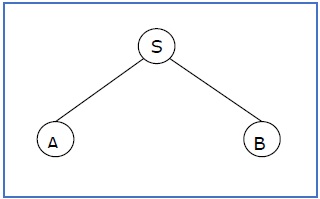
Se S → x 1 x 2 …… x n è una regola di produzione in un CFG, l'albero di analisi / albero di derivazione sarà il seguente:

Esistono due diversi approcci per disegnare un albero di derivazione:
Top-down Approach −
Inizia con il simbolo iniziale S
Scende alle foglie degli alberi usando le produzioni
Bottom-up Approach −
Inizia dalle foglie degli alberi
Procede verso l'alto fino alla radice che è il simbolo iniziale S
Derivazione o resa di un albero
La derivazione o la resa di un albero sintetico è la stringa finale ottenuta concatenando le etichette delle foglie dell'albero da sinistra a destra, ignorando i Nulli. Tuttavia, se tutte le foglie sono Null, la derivazione è Null.
Example
Sia un CFG {N, T, P, S}
N = {S}, T = {a, b}, simbolo iniziale = S, P = S → SS | aSb | ε
Una derivazione del CFG sopra è "abaabb"
S → SS → aSbS → abS → abaSb → abaaSbb → abaabb

Forma sentenziale e albero di derivazione parziale
Un albero di derivazione parziale è un sottoalbero di un albero di derivazione / albero sintetico in modo tale che tutti i suoi figli siano nel sottoalbero o nessuno di loro si trovi nel sottoalbero.
Example
Se in qualsiasi CFG le produzioni sono -
S → AB, A → aaA | ε, B → Bb | ε
l'albero di derivazione parziale può essere il seguente:
Se un albero di derivazione parziale contiene la radice S, viene chiamato a sentential form. Il sottoalbero di cui sopra è anche in forma sentenziale.
Derivazione più a sinistra e più a destra di una stringa
Leftmost derivation - Una derivazione più a sinistra si ottiene applicando la produzione alla variabile più a sinistra in ogni passaggio.
Rightmost derivation - Una derivazione più a destra si ottiene applicando la produzione alla variabile più a destra in ogni passaggio.
Example
Lascia che qualsiasi insieme di regole di produzione in un CFG sia
X → X + X | X * X | X | un
su un alfabeto {a}.
La derivazione più a sinistra per la stringa "a+a*a" può essere -
X → X + X → a + X → a + X * X → a + a * X → a + a * a
La derivazione graduale della stringa sopra è mostrata come di seguito:

La derivazione più a destra per la stringa precedente "a+a*a" può essere -
X → X * X → X * a → X + X * a → X + a * a → a + a * a
La derivazione graduale della stringa sopra è mostrata come di seguito:

Grammatiche ricorsive sinistra e destra
In una grammatica priva di contesto G, se c'è una produzione nella forma X → Xa dove X è un non terminale e ‘a’ è una stringa di terminali, si chiama a left recursive production. La grammatica che ha una produzione ricorsiva sinistra è chiamata aleft recursive grammar.
E se in una grammatica priva di contesto G, se c'è una produzione è nella forma X → aX dove X è un non terminale e ‘a’ è una stringa di terminali, si chiama a right recursive production. La grammatica che ha una produzione ricorsiva corretta è chiamata aright recursive grammar.
Se una grammatica libera dal contesto G ha più di un albero di derivazione per qualche stringa w ∈ L(G), si chiama un ambiguous grammar. Esistono più derivazioni più a destra o più a sinistra per alcune stringhe generate da quella grammatica.
Problema
Controlla se la grammatica G con le regole di produzione -
X → X + X | X * X | X | un
è ambiguo o no.
Soluzione
Scopriamo l'albero di derivazione per la stringa "a + a * a". Ha due derivazioni più a sinistra.
Derivation 1- X → X + X → a + X → a + X * X → a + a * X → a + a * a
Parse tree 1 -

Derivation 2- X → X * X → X + X * X → a + X * X → a + a * X → a + a * a
Parse tree 2 -

Poiché ci sono due alberi di analisi per una singola stringa "a + a * a", la grammatica G è ambiguo.
Le lingue prive di contesto sono closed sotto -
- Union
- Concatenation
- Operazione Kleene Star
Unione
Siano L 1 e L 2 due linguaggi privi di contesto. Allora L 1 ∪ L 2 è anch'esso libero dal contesto.
Esempio
Sia L 1 = {a n b n , n> 0}. La grammatica corrispondente G 1 avrà P: S1 → aAb | ab
Sia L 2 = {c m d m , m ≥ 0}. La grammatica corrispondente G 2 avrà P: S2 → cBb | ε
Unione di L 1 e L 2 , L = L 1 ∪ L 2 = {a n b n } ∪ {c m d m }
La grammatica corrispondente G avrà la produzione aggiuntiva S → S1 | S2
Concatenazione
Se L 1 e L 2 sono linguaggi privi di contesto, anche L 1 L 2 è privo di contesto.
Esempio
Unione delle lingue L 1 e L 2 , L = L 1 L 2 = {a n b n c m d m }
La grammatica corrispondente G avrà la produzione aggiuntiva S → S1 S2
Kleene Star
Se L è un linguaggio libero dal contesto, anche L * è libero dal contesto.
Esempio
Sia L = {a n b n , n ≥ 0}. La grammatica corrispondente G avrà P: S → aAb | ε
Kleene Star L 1 = {a n b n } *
La grammatica corrispondente G 1 avrà produzioni aggiuntive S1 → SS 1 | ε
Le lingue prive di contesto sono not closed sotto -
Intersection - Se L1 e L2 sono linguaggi privi di contesto, allora L1 ∩ L2 non è necessariamente privo di contesto.
Intersection with Regular Language - Se L1 è una lingua normale e L2 è una lingua libera dal contesto, allora L1 ∩ L2 è una lingua libera dal contesto.
Complement - Se L1 è un linguaggio libero dal contesto, allora L1 'potrebbe non essere libero dal contesto.
In un CFG, può accadere che tutte le regole e simboli di produzione non siano necessari per la derivazione di stringhe. Inoltre, potrebbero esserci alcune produzioni nulle e produzioni unitarie. Viene chiamata l'eliminazione di queste produzioni e simbolisimplification of CFGs. La semplificazione comprende essenzialmente i seguenti passaggi:
- Riduzione di CFG
- Rimozione delle produzioni unitarie
- Rimozione di produzioni nulle
Riduzione di CFG
I CFG vengono ridotti in due fasi:
Phase 1 - Derivazione di una grammatica equivalente, G’, dal CFG, G, in modo tale che ogni variabile derivi una stringa terminale.
Derivation Procedure -
Passaggio 1: includi tutti i simboli, W1, che derivano un terminale e inizializzano i=1.
Passaggio 2: includi tutti i simboli, Wi+1, che derivano Wi.
Passaggio 3: incremento i e ripetere il passaggio 2, finché Wi+1 = Wi.
Passaggio 4: includere tutte le regole di produzione che hanno Wi dentro.
Phase 2 - Derivazione di una grammatica equivalente, G”, dal CFG, G’, in modo tale che ogni simbolo appaia in una forma sentenziale.
Derivation Procedure -
Passaggio 1: includere il simbolo di inizio in Y1 e inizializza i = 1.
Passaggio 2: includi tutti i simboli, Yi+1, che può essere derivato da Yi e includere tutte le regole di produzione che sono state applicate.
Passaggio 3: incremento i e ripetere il passaggio 2, finché Yi+1 = Yi.
Problema
Trova una grammatica ridotta equivalente alla grammatica G, con regole di produzione, P: S → AC | B, A → a, C → c | BC, E → aA | e
Soluzione
Phase 1 -
T = {a, c, e}
W 1 = {A, C, E} dalle regole A → a, C → ce E → aA
W 2 = {A, C, E} U {S} dalla regola S → AC
W 3 = {LA, DO, MI, S} U ∅
Poiché W 2 = W 3 , possiamo derivare G 'come -
G '= {{A, C, E, S}, {a, c, e}, P, {S}}
dove P: S → AC, A → a, C → c, E → aA | e
Phase 2 -
Y 1 = {S}
Y 2 = {S, A, C} dalla regola S → AC
Y 3 = {S, A, C, a, c} dalle regole A → a e C → c
Y 4 = {S, A, C, a, c}
Poiché Y 3 = Y 4 , possiamo derivare G "come -
G "= {{A, C, S}, {a, c}, P, {S}}
dove P: S → AC, A → a, C → c
Rimozione delle produzioni unitarie
Qualsiasi regola di produzione nella forma A → B dove viene chiamata A, B ∈ Non terminale unit production..
Procedura di rimozione -
Step 1 - Per rimuovere A → B, add production A → x to the grammar rule whenever B → x occurs in the grammar. [x ∈ Terminal, x can be Null]
Step 2 − Delete A → B from the grammar.
Step 3 − Repeat from step 1 until all unit productions are removed.
Problem
Remove unit production from the following −
S → XY, X → a, Y → Z | b, Z → M, M → N, N → a
Solution −
There are 3 unit productions in the grammar −
Y → Z, Z → M, and M → N
At first, we will remove M → N.
As N → a, we add M → a, and M → N is removed.
The production set becomes
S → XY, X → a, Y → Z | b, Z → M, M → a, N → a
Now we will remove Z → M.
As M → a, we add Z→ a, and Z → M is removed.
The production set becomes
S → XY, X → a, Y → Z | b, Z → a, M → a, N → a
Now we will remove Y → Z.
As Z → a, we add Y→ a, and Y → Z is removed.
The production set becomes
S → XY, X → a, Y → a | b, Z → a, M → a, N → a
Now Z, M, and N are unreachable, hence we can remove those.
The final CFG is unit production free −
S → XY, X → a, Y → a | b
Removal of Null Productions
In a CFG, a non-terminal symbol ‘A’ is a nullable variable if there is a production A → ε or there is a derivation that starts at A and finally ends up with
ε: A → .......… → ε
Removal Procedure
Step 1 − Find out nullable non-terminal variables which derive ε.
Step 2 − For each production A → a, construct all productions A → x where x is obtained from ‘a’ by removing one or multiple non-terminals from Step 1.
Step 3 − Combine the original productions with the result of step 2 and remove ε - productions.
Problem
Remove null production from the following −
S → ASA | aB | b, A → B, B → b | ∈
Solution −
There are two nullable variables − A and B
At first, we will remove B → ε.
After removing B → ε, the production set becomes −
S→ASA | aB | b | a, A ε B| b | &epsilon, B → b
Now we will remove A → ε.
After removing A → ε, the production set becomes −
S→ASA | aB | b | a | SA | AS | S, A → B| b, B → b
This is the final production set without null transition.
A CFG is in Chomsky Normal Form if the Productions are in the following forms −
- A → a
- A → BC
- S → ε
where A, B, and C are non-terminals and a is terminal.
Algorithm to Convert into Chomsky Normal Form −
Step 1 − If the start symbol S occurs on some right side, create a new start symbol S’ and a new production S’→ S.
Step 2 − Remove Null productions. (Using the Null production removal algorithm discussed earlier)
Step 3 − Remove unit productions. (Using the Unit production removal algorithm discussed earlier)
Step 4 − Replace each production A → B1…Bn where n > 2 with A → B1C where C → B2 …Bn. Repeat this step for all productions having two or more symbols in the right side.
Step 5 − If the right side of any production is in the form A → aB where a is a terminal and A, B are non-terminal, then the production is replaced by A → XB and X → a. Repeat this step for every production which is in the form A → aB.
Problem
Convert the following CFG into CNF
S → ASA | aB, A → B | S, B → b | ε
Solution
(1) Since S appears in R.H.S, we add a new state S0 and S0→S is added to the production set and it becomes −
S0→S, S→ ASA | aB, A → B | S, B → b | ∈
(2) Now we will remove the null productions −
B → ∈ and A → ∈
After removing B → ε, the production set becomes −
S0→S, S→ ASA | aB | a, A → B | S | ∈, B → b
After removing A → ∈, the production set becomes −
S0→S, S→ ASA | aB | a | AS | SA | S, A → B | S, B → b
(3) Now we will remove the unit productions.
After removing S → S, the production set becomes −
S0→S, S→ ASA | aB | a | AS | SA, A → B | S, B → b
After removing S0→ S, the production set becomes −
S0→ ASA | aB | a | AS | SA, S→ ASA | aB | a | AS | SA
A → B | S, B → b
After removing A→ B, the production set becomes −
S0 → ASA | aB | a | AS | SA, S→ ASA | aB | a | AS | SA
A → S | b
B → b
After removing A→ S, the production set becomes −
S0 → ASA | aB | a | AS | SA, S→ ASA | aB | a | AS | SA
A → b |ASA | aB | a | AS | SA, B → b
(4) Now we will find out more than two variables in the R.H.S
Here, S0→ ASA, S → ASA, A→ ASA violates two Non-terminals in R.H.S.
Hence we will apply step 4 and step 5 to get the following final production set which is in CNF −
S0→ AX | aB | a | AS | SA
S→ AX | aB | a | AS | SA
A → b |AX | aB | a | AS | SA
B → b
X → SA
(5) We have to change the productions S0→ aB, S→ aB, A→ aB
And the final production set becomes −
S0→ AX | YB | a | AS | SA
S→ AX | YB | a | AS | SA
A → b A → b |AX | YB | a | AS | SA
B → b
X → SA
Y → a
A CFG is in Greibach Normal Form if the Productions are in the following forms −
A → b
A → bD1…Dn
S → ε
where A, D1,....,Dn are non-terminals and b is a terminal.
Algorithm to Convert a CFG into Greibach Normal Form
Step 1 − If the start symbol S occurs on some right side, create a new start symbol S’ and a new production S’ → S.
Step 2 − Remove Null productions. (Using the Null production removal algorithm discussed earlier)
Step 3 − Remove unit productions. (Using the Unit production removal algorithm discussed earlier)
Step 4 − Remove all direct and indirect left-recursion.
Step 5 − Do proper substitutions of productions to convert it into the proper form of GNF.
Problem
Convert the following CFG into CNF
S → XY | Xn | p
X → mX | m
Y → Xn | o
Solution
Here, S does not appear on the right side of any production and there are no unit or null productions in the production rule set. So, we can skip Step 1 to Step 3.
Step 4
Now after replacing
X in S → XY | Xo | p
with
mX | m
we obtain
S → mXY | mY | mXo | mo | p.
And after replacing
X in Y → Xn | o
with the right side of
X → mX | m
we obtain
Y → mXn | mn | o.
Two new productions O → o and P → p are added to the production set and then we came to the final GNF as the following −
S → mXY | mY | mXC | mC | p
X → mX | m
Y → mXD | mD | o
O → o
P → p
Lemma
If L is a context-free language, there is a pumping length p such that any string w ∈ L of length ≥ p can be written as w = uvxyz, where vy ≠ ε, |vxy| ≤ p, and for all i ≥ 0, uvixyiz ∈ L.
Applications of Pumping Lemma
Pumping lemma is used to check whether a grammar is context free or not. Let us take an example and show how it is checked.
Problem
Find out whether the language L = {xnynzn | n ≥ 1} is context free or not.
Solution
Let L is context free. Then, L must satisfy pumping lemma.
At first, choose a number n of the pumping lemma. Then, take z as 0n1n2n.
Break z into uvwxy, where
|vwx| ≤ n and vx ≠ ε.
Hence vwx cannot involve both 0s and 2s, since the last 0 and the first 2 are at least (n+1) positions apart. There are two cases −
Case 1 − vwx has no 2s. Then vx has only 0s and 1s. Then uwy, which would have to be in L, has n 2s, but fewer than n 0s or 1s.
Case 2 − vwx has no 0s.
Here contradiction occurs.
Hence, L is not a context-free language.
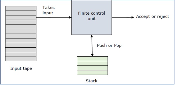
Basic Structure of PDA
A pushdown automaton is a way to implement a context-free grammar in a similar way we design DFA for a regular grammar. A DFA can remember a finite amount of information, but a PDA can remember an infinite amount of information.
Basically a pushdown automaton is −
"Finite state machine" + "a stack"
A pushdown automaton has three components −
- an input tape,
- a control unit, and
- a stack with infinite size.
The stack head scans the top symbol of the stack.
A stack does two operations −
Push − a new symbol is added at the top.
Pop − the top symbol is read and removed.
A PDA may or may not read an input symbol, but it has to read the top of the stack in every transition.
A PDA can be formally described as a 7-tuple (Q, ∑, S, δ, q0, I, F) −
Q is the finite number of states
∑ is input alphabet
S is stack symbols
δ is the transition function: Q × (∑ ∪ {ε}) × S × Q × S*
q0 is the initial state (q0 ∈ Q)
I is the initial stack top symbol (I ∈ S)
F is a set of accepting states (F ∈ Q)
The following diagram shows a transition in a PDA from a state q1 to state q2, labeled as a,b → c −
This means at state q1, if we encounter an input string ‘a’ and top symbol of the stack is ‘b’, then we pop ‘b’, push ‘c’ on top of the stack and move to state q2.
Terminologies Related to PDA
Instantaneous Description
The instantaneous description (ID) of a PDA is represented by a triplet (q, w, s) where
q is the state
w is unconsumed input
s is the stack contents
Turnstile Notation
The "turnstile" notation is used for connecting pairs of ID's that represent one or many moves of a PDA. The process of transition is denoted by the turnstile symbol "⊢".
Consider a PDA (Q, ∑, S, δ, q0, I, F). A transition can be mathematically represented by the following turnstile notation −
(p, aw, Tβ) ⊢ (q, w, αb)This implies that while taking a transition from state p to state q, the input symbol ‘a’ is consumed, and the top of the stack ‘T’ is replaced by a new string ‘α’.
Note − If we want zero or more moves of a PDA, we have to use the symbol (⊢*) for it.
There are two different ways to define PDA acceptability.
Final State Acceptability
In final state acceptability, a PDA accepts a string when, after reading the entire string, the PDA is in a final state. From the starting state, we can make moves that end up in a final state with any stack values. The stack values are irrelevant as long as we end up in a final state.
For a PDA (Q, ∑, S, δ, q0, I, F), the language accepted by the set of final states F is −
L(PDA) = {w | (q0, w, I) ⊢* (q, ε, x), q ∈ F}
for any input stack string x.
Empty Stack Acceptability
Here a PDA accepts a string when, after reading the entire string, the PDA has emptied its stack.
For a PDA (Q, ∑, S, δ, q0, I, F), the language accepted by the empty stack is −
L(PDA) = {w | (q0, w, I) ⊢* (q, ε, ε), q ∈ Q}
Example
Construct a PDA that accepts L = {0n 1n | n ≥ 0}
Solution

This language accepts L = {ε, 01, 0011, 000111, ............................. }
Here, in this example, the number of ‘a’ and ‘b’ have to be same.
Initially we put a special symbol ‘$’ into the empty stack.
Then at state q2, if we encounter input 0 and top is Null, we push 0 into stack. This may iterate. And if we encounter input 1 and top is 0, we pop this 0.
Then at state q3, if we encounter input 1 and top is 0, we pop this 0. This may also iterate. And if we encounter input 1 and top is 0, we pop the top element.
If the special symbol ‘$’ is encountered at top of the stack, it is popped out and it finally goes to the accepting state q4.
Example
Construct a PDA that accepts L = { wwR | w = (a+b)* }
Solution

Initially we put a special symbol ‘$’ into the empty stack. At state q2, the w is being read. In state q3, each 0 or 1 is popped when it matches the input. If any other input is given, the PDA will go to a dead state. When we reach that special symbol ‘$’, we go to the accepting state q4.
If a grammar G is context-free, we can build an equivalent nondeterministic PDA which accepts the language that is produced by the context-free grammar G. A parser can be built for the grammar G.
Also, if P is a pushdown automaton, an equivalent context-free grammar G can be constructed where
L(G) = L(P)
In the next two topics, we will discuss how to convert from PDA to CFG and vice versa.
Algorithm to find PDA corresponding to a given CFG
Input − A CFG, G = (V, T, P, S)
Output − Equivalent PDA, P = (Q, ∑, S, δ, q0, I, F)
Step 1 − Convert the productions of the CFG into GNF.
Step 2 − The PDA will have only one state {q}.
Step 3 − The start symbol of CFG will be the start symbol in the PDA.
Step 4 − All non-terminals of the CFG will be the stack symbols of the PDA and all the terminals of the CFG will be the input symbols of the PDA.
Step 5 − For each production in the form A → aX where a is terminal and A, X are combination of terminal and non-terminals, make a transition δ (q, a, A).
Problem
Construct a PDA from the following CFG.
G = ({S, X}, {a, b}, P, S)
where the productions are −
S → XS | ε , A → aXb | Ab | ab
Solution
Let the equivalent PDA,
P = ({q}, {a, b}, {a, b, X, S}, δ, q, S)
where δ −
δ(q, ε , S) = {(q, XS), (q, ε )}
δ(q, ε , X) = {(q, aXb), (q, Xb), (q, ab)}
δ(q, a, a) = {(q, ε )}
δ(q, 1, 1) = {(q, ε )}
Algorithm to find CFG corresponding to a given PDA
Input − A CFG, G = (V, T, P, S)
Output − Equivalent PDA, P = (Q, ∑, S, δ, q0, I, F) such that the non- terminals of the grammar G will be {Xwx | w,x ∈ Q} and the start state will be Aq0,F.
Step 1 − For every w, x, y, z ∈ Q, m ∈ S and a, b ∈ ∑, if δ (w, a, ε) contains (y, m) and (z, b, m) contains (x, ε), add the production rule Xwx → a Xyzb in grammar G.
Step 2 − For every w, x, y, z ∈ Q, add the production rule Xwx → XwyXyx in grammar G.
Step 3 − For w ∈ Q, add the production rule Xww → ε in grammar G.
Parsing is used to derive a string using the production rules of a grammar. It is used to check the acceptability of a string. Compiler is used to check whether or not a string is syntactically correct. A parser takes the inputs and builds a parse tree.
A parser can be of two types −
Top-Down Parser − Top-down parsing starts from the top with the start-symbol and derives a string using a parse tree.
Bottom-Up Parser − Bottom-up parsing starts from the bottom with the string and comes to the start symbol using a parse tree.
Design of Top-Down Parser
For top-down parsing, a PDA has the following four types of transitions −
Pop the non-terminal on the left hand side of the production at the top of the stack and push its right-hand side string.
If the top symbol of the stack matches with the input symbol being read, pop it.
Push the start symbol ‘S’ into the stack.
If the input string is fully read and the stack is empty, go to the final state ‘F’.
Example
Design a top-down parser for the expression "x+y*z" for the grammar G with the following production rules −
P: S → S+X | X, X → X*Y | Y, Y → (S) | id
Solution
If the PDA is (Q, ∑, S, δ, q0, I, F), then the top-down parsing is −
(x+y*z, I) ⊢(x +y*z, SI) ⊢ (x+y*z, S+XI) ⊢(x+y*z, X+XI)
⊢(x+y*z, Y+X I) ⊢(x+y*z, x+XI) ⊢(+y*z, +XI) ⊢ (y*z, XI)
⊢(y*z, X*YI) ⊢(y*z, y*YI) ⊢(*z,*YI) ⊢(z, YI) ⊢(z, zI) ⊢(ε, I)
Design of a Bottom-Up Parser
For bottom-up parsing, a PDA has the following four types of transitions −
Push the current input symbol into the stack.
Replace the right-hand side of a production at the top of the stack with its left-hand side.
If the top of the stack element matches with the current input symbol, pop it.
If the input string is fully read and only if the start symbol ‘S’ remains in the stack, pop it and go to the final state ‘F’.
Example
Design a top-down parser for the expression "x+y*z" for the grammar G with the following production rules −
P: S → S+X | X, X → X*Y | Y, Y → (S) | id
Solution
If the PDA is (Q, ∑, S, δ, q0, I, F), then the bottom-up parsing is −
(x+y*z, I) ⊢ (+y*z, xI) ⊢ (+y*z, YI) ⊢ (+y*z, XI) ⊢ (+y*z, SI)
⊢(y*z, +SI) ⊢ (*z, y+SI) ⊢ (*z, Y+SI) ⊢ (*z, X+SI) ⊢ (z, *X+SI)
⊢ (ε, z*X+SI) ⊢ (ε, Y*X+SI) ⊢ (ε, X+SI) ⊢ (ε, SI)
A Turing Machine is an accepting device which accepts the languages (recursively enumerable set) generated by type 0 grammars. It was invented in 1936 by Alan Turing.
Definition
A Turing Machine (TM) is a mathematical model which consists of an infinite length tape divided into cells on which input is given. It consists of a head which reads the input tape. A state register stores the state of the Turing machine. After reading an input symbol, it is replaced with another symbol, its internal state is changed, and it moves from one cell to the right or left. If the TM reaches the final state, the input string is accepted, otherwise rejected.
A TM can be formally described as a 7-tuple (Q, X, ∑, δ, q0, B, F) where −
Q is a finite set of states
X is the tape alphabet
∑ is the input alphabet
δ is a transition function; δ : Q × X → Q × X × {Left_shift, Right_shift}.
q0 is the initial state
B is the blank symbol
F is the set of final states
Comparison with the previous automaton
The following table shows a comparison of how a Turing machine differs from Finite Automaton and Pushdown Automaton.
| Machine | Stack Data Structure | Deterministic? |
|---|---|---|
| Finite Automaton | N.A | Yes |
| Pushdown Automaton | Last In First Out(LIFO) | No |
| Turing Machine | Infinite tape | Yes |
Example of Turing machine
Turing machine M = (Q, X, ∑, δ, q0, B, F) with
- Q = {q0, q1, q2, qf}
- X = {a, b}
- ∑ = {1}
- q0 = {q0}
- B = blank symbol
- F = {qf }
δ is given by −
| Tape alphabet symbol | Present State ‘q0’ | Present State ‘q1’ | Present State ‘q2’ |
|---|---|---|---|
| a | 1Rq1 | 1Lq0 | 1Lqf |
| b | 1Lq2 | 1Rq1 | 1Rqf |
Here the transition 1Rq1 implies that the write symbol is 1, the tape moves right, and the next state is q1. Similarly, the transition 1Lq2 implies that the write symbol is 1, the tape moves left, and the next state is q2.
Time and Space Complexity of a Turing Machine
For a Turing machine, the time complexity refers to the measure of the number of times the tape moves when the machine is initialized for some input symbols and the space complexity is the number of cells of the tape written.
Time complexity all reasonable functions −
T(n) = O(n log n)
TM's space complexity −
S(n) = O(n)
A TM accepts a language if it enters into a final state for any input string w. A language is recursively enumerable (generated by Type-0 grammar) if it is accepted by a Turing machine.
A TM decides a language if it accepts it and enters into a rejecting state for any input not in the language. A language is recursive if it is decided by a Turing machine.
There may be some cases where a TM does not stop. Such TM accepts the language, but it does not decide it.
Designing a Turing Machine
The basic guidelines of designing a Turing machine have been explained below with the help of a couple of examples.
Example 1
Design a TM to recognize all strings consisting of an odd number of α’s.
Solution
The Turing machine M can be constructed by the following moves −
Let q1 be the initial state.
If M is in q1; on scanning α, it enters the state q2 and writes B (blank).
If M is in q2; on scanning α, it enters the state q1 and writes B (blank).
From the above moves, we can see that M enters the state q1 if it scans an even number of α’s, and it enters the state q2 if it scans an odd number of α’s. Hence q2 is the only accepting state.
Hence,
M = {{q1, q2}, {1}, {1, B}, δ, q1, B, {q2}}
where δ is given by −
| Tape alphabet symbol | Present State ‘q1’ | Present State ‘q2’ |
|---|---|---|
| α | BRq2 | BRq1 |
Example 2
Design a Turing Machine that reads a string representing a binary number and erases all leading 0’s in the string. However, if the string comprises of only 0’s, it keeps one 0.
Solution
Let us assume that the input string is terminated by a blank symbol, B, at each end of the string.
The Turing Machine, M, can be constructed by the following moves −
Let q0 be the initial state.
If M is in q0, on reading 0, it moves right, enters the state q1 and erases 0. On reading 1, it enters the state q2 and moves right.
If M is in q1, on reading 0, it moves right and erases 0, i.e., it replaces 0’s by B’s. On reaching the leftmost 1, it enters q2 and moves right. If it reaches B, i.e., the string comprises of only 0’s, it moves left and enters the state q3.
If M is in q2, on reading either 0 or 1, it moves right. On reaching B, it moves left and enters the state q4. This validates that the string comprises only of 0’s and 1’s.
If M is in q3, it replaces B by 0, moves left and reaches the final state qf.
If M is in q4, on reading either 0 or 1, it moves left. On reaching the beginning of the string, i.e., when it reads B, it reaches the final state qf.
Hence,
M = {{q0, q1, q2, q3, q4, qf}, {0,1, B}, {1, B}, δ, q0, B, {qf}}
where δ is given by −
| Tape alphabet symbol | Present State ‘q0’ | Present State ‘q1’ | Present State ‘q2’ | Present State ‘q3’ | Present State ‘q4’ |
|---|---|---|---|---|---|
| 0 | BRq1 | BRq1 | ORq2 | - | OLq4 |
| 1 | 1Rq2 | 1Rq2 | 1Rq2 | - | 1Lq4 |
| B | BRq1 | BLq3 | BLq4 | OLqf | BRqf |
Multi-tape Turing Machines have multiple tapes where each tape is accessed with a separate head. Each head can move independently of the other heads. Initially the input is on tape 1 and others are blank. At first, the first tape is occupied by the input and the other tapes are kept blank. Next, the machine reads consecutive symbols under its heads and the TM prints a symbol on each tape and moves its heads.

A Multi-tape Turing machine can be formally described as a 6-tuple (Q, X, B, δ, q0, F) where −
Q is a finite set of states
X is the tape alphabet
B is the blank symbol
δ is a relation on states and symbols where
δ: Q × Xk → Q × (X × {Left_shift, Right_shift, No_shift })k
where there is k number of tapes
q0 is the initial state
F is the set of final states
Note − Every Multi-tape Turing machine has an equivalent single-tape Turing machine.
Multi-track Turing machines, a specific type of Multi-tape Turing machine, contain multiple tracks but just one tape head reads and writes on all tracks. Here, a single tape head reads n symbols from n tracks at one step. It accepts recursively enumerable languages like a normal single-track single-tape Turing Machine accepts.
A Multi-track Turing machine can be formally described as a 6-tuple (Q, X, ∑, δ, q0, F) where −
Q is a finite set of states
X is the tape alphabet
∑ is the input alphabet
δ is a relation on states and symbols where
δ(Qi, [a1, a2, a3,....]) = (Qj, [b1, b2, b3,....], Left_shift or Right_shift)
q0 is the initial state
F is the set of final states
Note − For every single-track Turing Machine S, there is an equivalent multi-track Turing Machine M such that L(S) = L(M).
In a Non-Deterministic Turing Machine, for every state and symbol, there are a group of actions the TM can have. So, here the transitions are not deterministic. The computation of a non-deterministic Turing Machine is a tree of configurations that can be reached from the start configuration.
An input is accepted if there is at least one node of the tree which is an accept configuration, otherwise it is not accepted. If all branches of the computational tree halt on all inputs, the non-deterministic Turing Machine is called a Decider and if for some input, all branches are rejected, the input is also rejected.
A non-deterministic Turing machine can be formally defined as a 6-tuple (Q, X, ∑, δ, q0, B, F) where −
Q is a finite set of states
X is the tape alphabet
∑ is the input alphabet
δ is a transition function;
δ : Q × X → P(Q × X × {Left_shift, Right_shift}).
q0 is the initial state
B is the blank symbol
F is the set of final states
A Turing Machine with a semi-infinite tape has a left end but no right end. The left end is limited with an end marker.

It is a two-track tape −
Upper track − It represents the cells to the right of the initial head position.
Lower track − It represents the cells to the left of the initial head position in reverse order.
The infinite length input string is initially written on the tape in contiguous tape cells.
The machine starts from the initial state q0 and the head scans from the left end marker ‘End’. In each step, it reads the symbol on the tape under its head. It writes a new symbol on that tape cell and then it moves the head either into left or right one tape cell. A transition function determines the actions to be taken.
It has two special states called accept state and reject state. If at any point of time it enters into the accepted state, the input is accepted and if it enters into the reject state, the input is rejected by the TM. In some cases, it continues to run infinitely without being accepted or rejected for some certain input symbols.
Note − Turing machines with semi-infinite tape are equivalent to standard Turing machines.
A linear bounded automaton is a multi-track non-deterministic Turing machine with a tape of some bounded finite length.
Length = function (Length of the initial input string, constant c)
Here,
Memory information ≤ c × Input information
The computation is restricted to the constant bounded area. The input alphabet contains two special symbols which serve as left end markers and right end markers which mean the transitions neither move to the left of the left end marker nor to the right of the right end marker of the tape.
A linear bounded automaton can be defined as an 8-tuple (Q, X, ∑, q0, ML, MR, δ, F) where −
Q is a finite set of states
X is the tape alphabet
∑ is the input alphabet
q0 is the initial state
ML is the left end marker
MR is the right end marker where MR ≠ ML
δ is a transition function which maps each pair (state, tape symbol) to (state, tape symbol, Constant ‘c’) where c can be 0 or +1 or -1
F is the set of final states

A deterministic linear bounded automaton is always context-sensitive and the linear bounded automaton with empty language is undecidable..
A language is called Decidable or Recursive if there is a Turing machine which accepts and halts on every input string w. Every decidable language is Turing-Acceptable.

A decision problem P is decidable if the language L of all yes instances to P is decidable.
For a decidable language, for each input string, the TM halts either at the accept or the reject state as depicted in the following diagram −

Example 1
Find out whether the following problem is decidable or not −
Is a number ‘m’ prime?
Solution
Prime numbers = {2, 3, 5, 7, 11, 13, …………..}
Divide the number ‘m’ by all the numbers between ‘2’ and ‘√m’ starting from ‘2’.
If any of these numbers produce a remainder zero, then it goes to the “Rejected state”, otherwise it goes to the “Accepted state”. So, here the answer could be made by ‘Yes’ or ‘No’.
Hence, it is a decidable problem.
Example 2
Given a regular language L and string w, how can we check if w ∈ L?
Solution
Take the DFA that accepts L and check if w is accepted

Some more decidable problems are −
- Does DFA accept the empty language?
- Is L1 ∩ L2 = ∅ for regular sets?
Note −
If a language L is decidable, then its complement L' is also decidable
If a language is decidable, then there is an enumerator for it.
For an undecidable language, there is no Turing Machine which accepts the language and makes a decision for every input string w (TM can make decision for some input string though). A decision problem P is called “undecidable” if the language L of all yes instances to P is not decidable. Undecidable languages are not recursive languages, but sometimes, they may be recursively enumerable languages.

Example
- The halting problem of Turing machine
- The mortality problem
- The mortal matrix problem
- The Post correspondence problem, etc.
Input − A Turing machine and an input string w.
Problem − Does the Turing machine finish computing of the string w in a finite number of steps? The answer must be either yes or no.
Proof − At first, we will assume that such a Turing machine exists to solve this problem and then we will show it is contradicting itself. We will call this Turing machine as a Halting machine that produces a ‘yes’ or ‘no’ in a finite amount of time. If the halting machine finishes in a finite amount of time, the output comes as ‘yes’, otherwise as ‘no’. The following is the block diagram of a Halting machine −

Now we will design an inverted halting machine (HM)’ as −
If H returns YES, then loop forever.
If H returns NO, then halt.
The following is the block diagram of an ‘Inverted halting machine’ −

Further, a machine (HM)2 which input itself is constructed as follows −
- If (HM)2 halts on input, loop forever.
- Else, halt.
Here, we have got a contradiction. Hence, the halting problem is undecidable.
Rice theorem states that any non-trivial semantic property of a language which is recognized by a Turing machine is undecidable. A property, P, is the language of all Turing machines that satisfy that property.
Formal Definition
If P is a non-trivial property, and the language holding the property, Lp , is recognized by Turing machine M, then Lp = {<M> | L(M) ∈ P} is undecidable.
Description and Properties
Property of languages, P, is simply a set of languages. If any language belongs to P (L ∈ P), it is said that L satisfies the property P.
A property is called to be trivial if either it is not satisfied by any recursively enumerable languages, or if it is satisfied by all recursively enumerable languages.
A non-trivial property is satisfied by some recursively enumerable languages and are not satisfied by others. Formally speaking, in a non-trivial property, where L ∈ P, both the following properties hold:
Property 1 − There exists Turing Machines, M1 and M2 that recognize the same language, i.e. either ( <M1>, <M2> ∈ L ) or ( <M1>,<M2> ∉ L )
Property 2 − There exists Turing Machines M1 and M2, where M1 recognizes the language while M2 does not, i.e. <M1> ∈ L and <M2> ∉ L
Proof
Suppose, a property P is non-trivial and φ ∈ P.
Since, P is non-trivial, at least one language satisfies P, i.e., L(M0) ∈ P , ∋ Turing Machine M0.
Let, w be an input in a particular instant and N is a Turing Machine which follows −
On input x
- Run M on w
- If M does not accept (or doesn't halt), then do not accept x (or do not halt)
- If M accepts w then run M0 on x. If M0 accepts x, then accept x.
A function that maps an instance ATM = {<M,w>| M accepts input w} to a N such that
- If M accepts w and N accepts the same language as M0, Then L(M) = L(M0) ∈ p
- If M does not accept w and N accepts φ, Then L(N) = φ ∉ p
Since ATM is undecidable and it can be reduced to Lp, Lp is also undecidable.
The Post Correspondence Problem (PCP), introduced by Emil Post in 1946, is an undecidable decision problem. The PCP problem over an alphabet ∑ is stated as follows −
Given the following two lists, M and N of non-empty strings over ∑ −
M = (x1, x2, x3,………, xn)
N = (y1, y2, y3,………, yn)
We can say that there is a Post Correspondence Solution, if for some i1,i2,………… ik, where 1 ≤ ij ≤ n, the condition xi1 …….xik = yi1 …….yik satisfies.
Example 1
Find whether the lists
M = (abb, aa, aaa) and N = (bba, aaa, aa)
have a Post Correspondence Solution?
Solution
| x1 | x2 | x3 | |
|---|---|---|---|
| M | Abb | aa | aaa |
| N | Bba | aaa | aa |
Here,
x2x1x3 = ‘aaabbaaa’
and y2y1y3 = ‘aaabbaaa’
We can see that
x2x1x3 = y2y1y3
Hence, the solution is i = 2, j = 1, and k = 3.
Example 2
Find whether the lists M = (ab, bab, bbaaa) and N = (a, ba, bab) have a Post Correspondence Solution?
Solution
| x1 | x2 | x3 | |
|---|---|---|---|
| M | ab | bab | bbaaa |
| N | a | ba | bab |
In this case, there is no solution because −
| x2x1x3 | ≠ | y2y1y3 | (Lengths are not same)
Hence, it can be said that this Post Correspondence Problem is undecidable.