빅 데이터 분석-데이터 탐색
Exploratory data analysis통계의 새로운 관점으로 구성된 John Tuckey (1977)가 개발 한 개념입니다. Tuckey의 아이디어는 전통적인 통계에서 데이터가 그래픽으로 탐색되지 않고 가설을 테스트하는 데 사용된다는 것입니다. 도구를 개발하려는 첫 번째 시도는 스탠포드에서 이루어 졌으며이 프로젝트는 prim9 라고 불 렸습니다 . 이 도구는 데이터를 9 개 차원으로 시각화 할 수 있었으므로 데이터에 대한 다 변수 관점을 제공 할 수있었습니다.
최근에는 탐색 적 데이터 분석이 필수이며 빅 데이터 분석 수명주기에 포함되었습니다. 통찰력을 찾고 조직 내에서 효과적으로 소통 할 수있는 능력은 강력한 EDA 기능을 통해 촉진됩니다.
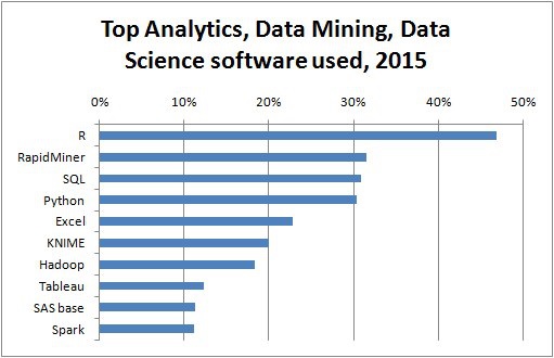
Tuckey의 아이디어를 바탕으로 Bell Labs는 S programming language통계를 수행하기위한 대화 형 인터페이스를 제공하기 위해. S의 아이디어는 사용하기 쉬운 언어로 광범위한 그래픽 기능을 제공하는 것이 었습니다. 오늘날의 세계에서 빅 데이터의 맥락에서R 그 기반 S 프로그래밍 언어는 분석에 가장 많이 사용되는 소프트웨어입니다.
다음 프로그램은 탐색 적 데이터 분석의 사용을 보여줍니다.
다음은 탐색 적 데이터 분석의 예입니다. 이 코드는part1/eda/exploratory_data_analysis.R 파일.
library(nycflights13)
library(ggplot2)
library(data.table)
library(reshape2)

# Using the code from the previous section
# This computes the mean arrival and departure delays by carrier.
DT <- as.data.table(flights)
mean2 = DT[, list(mean_departure_delay = mean(dep_delay, na.rm = TRUE),
   mean_arrival_delay = mean(arr_delay, na.rm = TRUE)),
   by = carrier]

# In order to plot data in R usign ggplot, it is normally needed to reshape the data
# We want to have the data in long format for plotting with ggplot
dt = melt(mean2, id.vars = ’carrier’)

# Take a look at the first rows
print(head(dt))

# Take a look at the help for ?geom_point and geom_line to find similar examples
# Here we take the carrier code as the x axis
# the value from the dt data.table goes in the y axis

# The variable column represents the color
p = ggplot(dt, aes(x = carrier, y = value, color = variable, group = variable)) +
   geom_point() + # Plots points
   geom_line() + # Plots lines
   theme_bw() + # Uses a white background
   labs(list(title = 'Mean arrival and departure delay by carrier',
      x = 'Carrier', y = 'Mean delay'))
print(p)

# Save the plot to disk
ggsave('mean_delay_by_carrier.png', p,
   width = 10.4, height = 5.07)
코드는 다음과 같은 이미지를 생성해야합니다.
