ऑटोमेटा सिद्धांत - त्वरित गाइड

ऑटोमेटा - यह क्या है?

"ऑटोमेटा" शब्द ग्रीक शब्द "ατμα "α" से लिया गया है जिसका अर्थ है "आत्म-अभिनय"। एक ऑटोमेटन (बहुवचन में स्वचालित) एक अमूर्त स्व-चालित कंप्यूटिंग डिवाइस है जो स्वचालित रूप से संचालन के पूर्व निर्धारित अनुक्रम का अनुसरण करता है।

राज्यों की एक परिमित संख्या के साथ एक ऑटोमेटन एक कहा जाता है Finite Automaton (एफए) या Finite State Machine (FSM)।

एक Finite Automaton की औपचारिक परिभाषा

एक ऑटोमेटन को 5-ट्यूपल (Q, represented, q, q ₀ , F) द्वारा दर्शाया जा सकता है , जहां -

Q राज्यों का एक समुच्चय है।
∑ प्रतीकों का एक परिमित सेट है, जिसे कहा जाता है alphabet ऑटोमेटन का।
δ संक्रमण कार्य है।
q₀वह प्रारंभिक अवस्था है जहां से किसी भी इनपुट को संसाधित किया जाता है (q ₀ ) Q)।
F अंतिम स्थिति / Q (F। Q) के राज्यों का एक समूह है।

निर्धारक परिमित ऑटोमेटन (DFA)

डीएफए में, प्रत्येक इनपुट प्रतीक के लिए, कोई व्यक्ति यह निर्धारित कर सकता है कि मशीन किस दिशा में जाएगी। इसलिए, इसे कहा जाता हैDeterministic Automaton। जैसा कि इसमें राज्यों की एक सीमित संख्या है, मशीन कहा जाता हैDeterministic Finite Machine या Deterministic Finite Automaton.

DFA की औपचारिक परिभाषा

एक डीएफए का प्रतिनिधित्व 5-ट्यूपल (क्यू, represented, q, q ₀ , F) द्वारा किया जा सकता है , जहां -

Q राज्यों का एक समुच्चय है।
∑ वर्णमाला नामक प्रतीकों का एक परिमित समुच्चय है।
δ वह संक्रमण क्रिया है जहाँ δ: Q ×। → Q
q₀वह प्रारंभिक अवस्था है जहां से किसी भी इनपुट को संसाधित किया जाता है (q ₀ ) Q)।
F अंतिम स्थिति / Q (F। Q) के राज्यों का एक समूह है।

एक डीएफए के चित्रमय प्रतिनिधित्व

एक डीएफए को डिग्राफ्स द्वारा दर्शाया जाता है state diagram।

कोने राज्यों का प्रतिनिधित्व करते हैं।
इनपुट वर्णमाला के साथ लेबल किए गए आर्क्स संक्रमण दिखाते हैं।
प्रारंभिक अवस्था को एक खाली आवक चाप द्वारा निरूपित किया जाता है।
अंतिम अवस्था को दोहरे वृत्तों द्वारा इंगित किया जाता है।

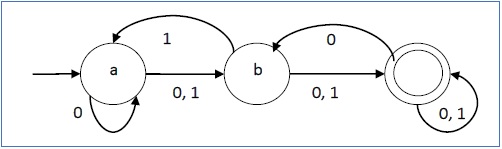
उदाहरण

एक नियत परिमित ऑटोमोटन होने दें →

क्यू = {ए, बी, सी},
, = {0, 1},
q ₀ = {a},
एफ = {सी}, और

संक्रमण कार्य δ जैसा कि निम्नलिखित तालिका द्वारा दिखाया गया है -

वर्तमान स्थिति	इनपुट के लिए अगला राज्य 0	इनपुट के लिए अगला राज्य 1
a	ए	ख
b	सी	ए
c	ख	सी

इसका ग्राफिकल प्रतिनिधित्व इस प्रकार होगा -

NDFA में, एक विशेष इनपुट प्रतीक के लिए, मशीन मशीन में राज्यों के किसी भी संयोजन को स्थानांतरित कर सकती है। दूसरे शब्दों में, मशीन ले जाने के लिए सटीक स्थिति निर्धारित नहीं की जा सकती। इसलिए, इसे कहा जाता हैNon-deterministic Automaton। जैसा कि इसमें राज्यों की सीमित संख्या है, मशीन को कहा जाता हैNon-deterministic Finite Machine या Non-deterministic Finite Automaton।

एक NDFA की औपचारिक परिभाषा

एक एनडीएफए का प्रतिनिधित्व 5-ट्यूपल (क्यू, represented, represented, q ₀ , F) द्वारा किया जा सकता है , जहां -

Q राज्यों का एक समुच्चय है।
∑ प्रतीकों का एक छोटा सेट है जिसे अक्षर कहा जाता है।
δसंक्रमण समारोह है जहां δ: Q × Q → 2 ^Q

(यहां क्यू (2 ^क्यू ) का पावर सेट लिया गया है क्योंकि एनडीएफए के मामले में, एक राज्य से, क्यू राज्यों के किसी भी संयोजन में संक्रमण हो सकता है)
q₀वह प्रारंभिक अवस्था है जहां से किसी भी इनपुट को संसाधित किया जाता है (q ₀ ) Q)।
F अंतिम स्थिति / Q (F। Q) के राज्यों का एक समूह है।

एक NDFA का चित्रमय प्रतिनिधित्व: (DFA के समान)

एनडीएफए को राज्य आरेख नामक डिग्राफ द्वारा दर्शाया जाता है।

कोने राज्यों का प्रतिनिधित्व करते हैं।
इनपुट वर्णमाला के साथ लेबल किए गए आर्क्स संक्रमण दिखाते हैं।
प्रारंभिक अवस्था को एक खाली आवक चाप द्वारा निरूपित किया जाता है।
अंतिम अवस्था को दोहरे वृत्तों द्वारा इंगित किया जाता है।

Example

एक गैर-नियतात्मक परिमित ऑटोमेटन होने दें →

क्यू = {ए, बी, सी}
, = {0, 1}
q ₀ = {a}
F = {c}

संक्रमण समारोह transition जैसा कि नीचे दिखाया गया है -

वर्तमान स्थिति	इनपुट के लिए अगला राज्य 0	इनपुट के लिए अगला राज्य 1
ए	ए, बी	ख
ख	सी	एसी
सी	बी, सी	सी

इसका ग्राफिकल प्रतिनिधित्व इस प्रकार होगा -

DFA बनाम NDFA

निम्न तालिका डीएफए और एनडीएफए के बीच के अंतरों को सूचीबद्ध करती है।

DFA	NDFA
एक राज्य से संक्रमण प्रत्येक इनपुट प्रतीक के लिए एक विशेष अगले राज्य के लिए है। इसलिए इसे नियतात्मक कहा जाता है ।	एक राज्य से संक्रमण प्रत्येक इनपुट प्रतीक के लिए कई अगले राज्यों में हो सकता है। इसलिए इसे गैर-नियतात्मक कहा जाता है ।
डीएफए में खाली स्ट्रिंग संक्रमण नहीं देखा जाता है।	NDFA खाली स्ट्रिंग संक्रमण की अनुमति देता है।
DFA में बैकट्रैकिंग की अनुमति है	NDFA में, बैकट्रैकिंग हमेशा संभव नहीं होता है।
अधिक स्थान की आवश्यकता है।	कम जगह चाहिए।
एक स्ट्रिंग को डीएफए द्वारा स्वीकार किया जाता है, अगर यह एक अंतिम स्थिति में स्थानांतरित होता है।	एक स्ट्रिंग एक NDFA द्वारा स्वीकार की जाती है, यदि अंतिम अवस्था में सभी संभावित संक्रमणों में से कम से कम एक समाप्त हो जाती है।

स्वीकर्ता, क्लासिफायर और ट्रांसड्यूसर

स्वीकर्ता (पहचानकर्ता)

एक ऑटोमेटन जो एक बूलियन फ़ंक्शन की गणना करता है, एक कहा जाता है acceptor। एक स्वीकर्ता के सभी राज्य या तो दिए गए इनपुट को स्वीकार या अस्वीकार कर रहे हैं।

वर्गीकरणकर्ता

ए classifier दो से अधिक अंतिम अवस्थाएं हैं और यह समाप्त होने पर एकल आउटपुट देता है।

ट्रांसड्यूसर

एक ऑटोमेटन जो वर्तमान इनपुट और / या पिछली स्थिति के आधार पर आउटपुट उत्पन्न करता है, a कहलाता है transducer। ट्रांसड्यूसर दो प्रकार के हो सकते हैं -

Mealy Machine - आउटपुट वर्तमान स्थिति और वर्तमान इनपुट दोनों पर निर्भर करता है।
Moore Machine - आउटपुट केवल वर्तमान स्थिति पर निर्भर करता है।

DFA और NDFA द्वारा स्वीकार्यता

एक स्ट्रिंग को डीएफए / एनडीएफए द्वारा स्वीकार किया जाता है यदि प्रारंभिक अवस्था में शुरू होने वाले डीएफए / एनडीएफए स्ट्रिंग को पूरी तरह से पढ़ने के बाद एक स्वीकृत राज्य (अंतिम राज्यों में से कोई भी) समाप्त होता है।

एक स्ट्रिंग S को DFA / NDFA (Q, δ, q, q ₀ , F), iff द्वारा स्वीकार किया जाता है

δ*(q₀, S) ∈ F

भाषा L DFA / NDFA द्वारा स्वीकार किया जाता है

{S | S ∈ ∑* and δ*(q₀, S) ∈ F}

एक स्ट्रिंग S ND को DFA / NDFA (Q, δ, ′, q ₀ , F), iff द्वारा स्वीकार नहीं किया जाता है

δ*(q₀, S′) ∉ F

डीएफए / एनडीएफए (स्वीकृत भाषा एल का पूरक) द्वारा स्वीकृत भाषा The नहीं है

{S | S ∈ ∑* and δ*(q₀, S) ∉ F}

Example

आइए हम चित्र 1.3 में दिखाए गए डीएफए पर विचार करें। DFA से स्वीकार्य तार निकाले जा सकते हैं।

उपरोक्त DFA द्वारा स्वीकृत स्ट्रिंग्स: {0, 00, 11, 010, 101, ...........}

उपरोक्त DFA द्वारा स्वीकार नहीं किए गए स्ट्रिंग्स: {1, 011, 111, ........}

समस्या का विवरण

लश्कर X = (Q_x, ∑, δ_x, q₀, F_x)एक NDFA बनें जो L (X) भाषा को स्वीकार करता है। हमें एक समतुल्य डीएफए डिजाइन करना होगाY = (Q_y, ∑, δ_y, q₀, F_y) ऐसा है कि L(Y) = L(X)। निम्नलिखित प्रक्रिया NDFA को उसके समकक्ष DFA में परिवर्तित करती है -

कलन विधि

Input - एक NDFA

Output - समतुल्य डीएफए

Step 1 - दिए गए एनडीएफए से राज्य तालिका बनाएं।

Step 2 - समतुल्य डीएफए के लिए संभावित इनपुट अल्फाबेट्स के तहत एक खाली राज्य तालिका बनाएं।

Step 3 - क्यूए (एक ही NDFA के रूप में) द्वारा DFA के प्रारंभ राज्य को चिह्नित करें।

Step 4- प्रत्येक संभावित इनपुट वर्णमाला के लिए राज्यों {Q ₀ , Q ₁ , ..., Q _n } के संयोजन का पता लगाएं ।

Step 5 - हर बार जब हम इनपुट वर्णमाला कॉलम के तहत एक नया डीएफए राज्य बनाते हैं, तो हमें चरण 4 को फिर से लागू करना होगा, अन्यथा चरण 6 पर जाएं।

Step 6 - जिन राज्यों में NDFA के अंतिम राज्यों में से कोई भी शामिल है, वे समान DFA के अंतिम राज्य हैं।

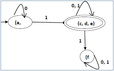
उदाहरण

आइए नीचे दिए गए आंकड़े में दिखाए गए एनडीएफए पर विचार करें।

क्यू	δ (क्यू, 0)	δ (क्यू, 1)
ए	{A, b, सी, डी, ई}	{डे}
ख	{सी}	{इ}
सी	∅	{B}
घ	{इ}	∅
इ	∅	∅

उपरोक्त एल्गोरिथ्म का उपयोग करते हुए, हम इसके समकक्ष डीएफए पाते हैं। डीएफए की राज्य तालिका नीचे दी गई है।

क्यू	δ (क्यू, 0)	δ (क्यू, 1)
[ए]	[ए, बी, सी, डी, ई]	[डे]
[ए, बी, सी, डी, ई]	[ए, बी, सी, डी, ई]	[ख, डी, ई]
[डे]	[इ]	∅
[ख, डी, ई]	[सी, ई]	[इ]
[इ]	∅	∅
[सी, ई]	∅	[ख]
[ख]	[सी]	[इ]
[सी]	∅	[ख]

डीएफए का राज्य चित्र इस प्रकार है -

DFA मिनीमाइज़ेशन का उपयोग करके Myhill-Nerode प्रमेय

कलन विधि

Input - डीएफए

Output - न्यूनतम डीएफए

Step 1- सभी राज्यों की जोड़ी के लिए एक तालिका बनाएं (क्यू _मैं , क्यू _जे ) जरूरी नहीं कि सीधे जुड़े हों [सभी शुरू में ही अप्रकाशित हैं]

Step 2- डीएफए में प्रत्येक राज्य जोड़ी (क्यू _आई , क्यू _जे ) पर विचार करें जहां क्यू _मैं Q एफ और क्यू _जे a एफ या इसके विपरीत और उन्हें चिह्नित करता हूं। [यहाँ एफ अंतिम राज्यों का सेट है]

Step 3 - इस चरण को तब तक दोहराएं, जब तक कि हम अब और चिह्नित नहीं कर सकते -

यदि कोई अचिह्नित जोड़ा (Q _i , Q _j ) है, तो इसे चिह्नित करें यदि जोड़ी {δ (Q _i , A), A (Q _i , A)} कुछ इनपुट वर्णमाला के लिए चिह्नित है।

Step 4- सभी अचिह्नित जोड़ी (Q _i , Q _j ) को मिलाएं और उन्हें कम DFA में एक एकल राज्य बनाएं।

उदाहरण

आइए नीचे दिखाए गए DFA को कम करने के लिए Algorithm 2 का उपयोग करें।

Step 1 - हम सभी राज्यों की जोड़ी के लिए एक तालिका बनाते हैं।

	ए	ख	सी	घ	इ	च
ए
ख
सी
घ
इ
च

Step 2 - हम राज्य जोड़े को चिह्नित करते हैं।

	ए	ख	सी	घ	इ	च
ए
ख
सी	✔	✔
घ	✔	✔
इ	✔	✔
च			✔	✔	✔

Step 3- हम राज्य के जोड़े को हरे रंग के चेक मार्क के साथ, संक्रमणीय रूप से चिह्नित करने का प्रयास करेंगे। यदि हम 1 को 'a' और 'f' को स्टेट करते हैं, तो यह क्रमशः 'c' और 'f' पर जाएगा। (सी, एफ) पहले से ही चिह्नित है, इसलिए हम जोड़ी (ए, एफ) को चिह्नित करेंगे। अब, हम 1 से 'b' और 'f' स्टेट इनपुट करते हैं; यह क्रमशः 'd' और 'f' राज्य में जाएगा। (डी, एफ) पहले से ही चिह्नित है, इसलिए हम जोड़ी (बी, एफ) को चिह्नित करेंगे।

	a	b	c	d	e	f
a
b
c	✔	✔
d	✔	✔
e	✔	✔
f	✔	✔	✔	✔	✔

After step 3, we have got state combinations {a, b} {c, d} {c, e} {d, e} that are unmarked.

We can recombine {c, d} {c, e} {d, e} into {c, d, e}

Hence we got two combined states as − {a, b} and {c, d, e}

So the final minimized DFA will contain three states {f}, {a, b} and {c, d, e}

DFA Minimization using Equivalence Theorem

If X and Y are two states in a DFA, we can combine these two states into {X, Y} if they are not distinguishable. Two states are distinguishable, if there is at least one string S, such that one of δ (X, S) and δ (Y, S) is accepting and another is not accepting. Hence, a DFA is minimal if and only if all the states are distinguishable.

Algorithm 3

Step 1 − All the states Q are divided in two partitions − final states and non-final states and are denoted by P₀. All the states in a partition are 0^th equivalent. Take a counter k and initialize it with 0.

Step 2 − Increment k by 1. For each partition in P_k, divide the states in P_k into two partitions if they are k-distinguishable. Two states within this partition X and Y are k-distinguishable if there is an input S such that δ(X, S) and δ(Y, S) are (k-1)-distinguishable.

Step 3 − If P_k ≠ P_k-1, repeat Step 2, otherwise go to Step 4.

Step 4 − Combine k^th equivalent sets and make them the new states of the reduced DFA.

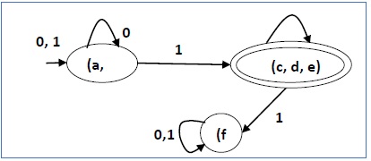
Example

Let us consider the following DFA −

q	δ(q,0)	δ(q,1)
a	b	c
b	a	d
c	e	f
d	e	f
e	e	f
f	f	f

Let us apply the above algorithm to the above DFA −

P₀ = {(c,d,e), (a,b,f)}
P₁ = {(c,d,e), (a,b),(f)}
P₂ = {(c,d,e), (a,b),(f)}

Hence, P₁ = P₂.

There are three states in the reduced DFA. The reduced DFA is as follows −

Q	δ(q,0)	δ(q,1)
(a, b)	(a, b)	(c,d,e)
(c,d,e)	(c,d,e)	(f)
(f)	(f)	(f)

Finite automata may have outputs corresponding to each transition. There are two types of finite state machines that generate output −

Mealy Machine
Moore machine

Mealy Machine

A Mealy Machine is an FSM whose output depends on the present state as well as the present input.

It can be described by a 6 tuple (Q, ∑, O, δ, X, q₀) where −

Q is a finite set of states.
∑ is a finite set of symbols called the input alphabet.
O is a finite set of symbols called the output alphabet.
δ is the input transition function where δ: Q × ∑ → Q
X is the output transition function where X: Q × ∑ → O
q₀ is the initial state from where any input is processed (q₀ ∈ Q).

The state table of a Mealy Machine is shown below −

Present state	Next state
	input = 0		input = 1
	State	Output	State	Output
→ a	b	x₁	c	x₁
b	b	x₂	d	x₃
c	d	x₃	c	x₁
d	d	x₃	d	x₂

The state diagram of the above Mealy Machine is −

Moore Machine

Moore machine is an FSM whose outputs depend on only the present state.

A Moore machine can be described by a 6 tuple (Q, ∑, O, δ, X, q₀) where −

Q is a finite set of states.
∑ is a finite set of symbols called the input alphabet.
O is a finite set of symbols called the output alphabet.
δ is the input transition function where δ: Q × ∑ → Q
X is the output transition function where X: Q → O
q₀ is the initial state from where any input is processed (q₀ ∈ Q).

The state table of a Moore Machine is shown below −

Present state	Next State		Output
Present state	Input = 0	Input = 1	Output
→ a	b	c	x₂
b	b	d	x₁
c	c	d	x₂
d	d	d	x₃

The state diagram of the above Moore Machine is −

Mealy Machine vs. Moore Machine

The following table highlights the points that differentiate a Mealy Machine from a Moore Machine.

Mealy Machine	Moore Machine
Output depends both upon the present state and the present input	Output depends only upon the present state.
Generally, it has fewer states than Moore Machine.	Generally, it has more states than Mealy Machine.
The value of the output function is a function of the transitions and the changes, when the input logic on the present state is done.	The value of the output function is a function of the current state and the changes at the clock edges, whenever state changes occur.
Mealy machines react faster to inputs. They generally react in the same clock cycle.	In Moore machines, more logic is required to decode the outputs resulting in more circuit delays. They generally react one clock cycle later.

Moore Machine to Mealy Machine

Algorithm 4

Input − Moore Machine

Output − Mealy Machine

Step 1 − Take a blank Mealy Machine transition table format.

Step 2 − Copy all the Moore Machine transition states into this table format.

Step 3 − Check the present states and their corresponding outputs in the Moore Machine state table; if for a state Q_i output is m, copy it into the output columns of the Mealy Machine state table wherever Q_i appears in the next state.

Example

Let us consider the following Moore machine −

Present State	Next State		Output
Present State	a = 0	a = 1	Output
→ a	d	b	1
b	a	d	0
c	c	c	0
d	b	a	1

Now we apply Algorithm 4 to convert it to Mealy Machine.

Step 1 & 2 −

Present State	Next State
	a = 0		a = 1
	State	Output	State	Output
→ a	d		b
b	a		d
c	c		c
d	b		a

Step 3 −

Present State	Next State
	a = 0		a = 1
	State	Output	State	Output
=> a	d	1	b	0
b	a	1	d	1
c	c	0	c	0
d	b	0	a	1

Mealy Machine to Moore Machine

Algorithm 5

Input − Mealy Machine

Output − Moore Machine

Step 1 − Calculate the number of different outputs for each state (Q_i) that are available in the state table of the Mealy machine.

Step 2 − If all the outputs of Qi are same, copy state Q_i. If it has n distinct outputs, break Q_i into n states as Q_in where n = 0, 1, 2.......

Step 3 − If the output of the initial state is 1, insert a new initial state at the beginning which gives 0 output.

Example

Let us consider the following Mealy Machine −

Present State	Next State
	a = 0		a = 1
	Next State	Output	Next State	Output
→ a	d	0	b	1
b	a	1	d	0
c	c	1	c	0
d	b	0	a	1

Here, states ‘a’ and ‘d’ give only 1 and 0 outputs respectively, so we retain states ‘a’ and ‘d’. But states ‘b’ and ‘c’ produce different outputs (1 and 0). So, we divide b into b₀, b₁ and c into c₀, c₁.

Present State	Next State		Output
Present State	a = 0	a = 1	Output
→ a	d	b₁	1
b₀	a	d	0
b₁	a	d	1
c₀	c₁	C₀	0
c₁	c₁	C₀	1
d	b₀	a	0

n the literary sense of the term, grammars denote syntactical rules for conversation in natural languages. Linguistics have attempted to define grammars since the inception of natural languages like English, Sanskrit, Mandarin, etc.

The theory of formal languages finds its applicability extensively in the fields of Computer Science. Noam Chomsky gave a mathematical model of grammar in 1956 which is effective for writing computer languages.

Grammar

A grammar G can be formally written as a 4-tuple (N, T, S, P) where −

N or V_N is a set of variables or non-terminal symbols.
T or ∑ is a set of Terminal symbols.
S is a special variable called the Start symbol, S ∈ N
P is Production rules for Terminals and Non-terminals. A production rule has the form α → β, where α and β are strings on V_N ∪ ∑ and least one symbol of α belongs to V_N.

Example

Grammar G1 −

({S, A, B}, {a, b}, S, {S → AB, A → a, B → b})

Here,

S, A, and B are Non-terminal symbols;
a and b are Terminal symbols
S is the Start symbol, S ∈ N
Productions, P : S → AB, A → a, B → b

Example

Grammar G2 −

(({S, A}, {a, b}, S,{S → aAb, aA → aaAb, A → ε } )

Here,

S and A are Non-terminal symbols.
a and b are Terminal symbols.
ε is an empty string.
S is the Start symbol, S ∈ N
Production P : S → aAb, aA → aaAb, A → ε

Derivations from a Grammar

Strings may be derived from other strings using the productions in a grammar. If a grammar G has a production α → β, we can say that x α y derives x β y in G. This derivation is written as −

x α y ⇒G x β y

Example

Let us consider the grammar −

G2 = ({S, A}, {a, b}, S, {S → aAb, aA → aaAb, A → ε } )

Some of the strings that can be derived are −

S ⇒ aAb using production S → aAb

⇒ aaAbb using production aA → aAb

⇒ aaaAbbb using production aA → aAb

⇒ aaabbb using production A → ε

The set of all strings that can be derived from a grammar is said to be the language generated from that grammar. A language generated by a grammar G is a subset formally defined by

L(G)={W|W ∈ ∑*, S ⇒G W}

If L(G1) = L(G2), the Grammar G1 is equivalent to the Grammar G2.

Example

If there is a grammar

G: N = {S, A, B} T = {a, b} P = {S → AB, A → a, B → b}

Here S produces AB, and we can replace A by a, and B by b. Here, the only accepted string is ab, i.e.,

L(G) = {ab}

Example

Suppose we have the following grammar −

G: N = {S, A, B} T = {a, b} P = {S → AB, A → aA|a, B → bB|b}

The language generated by this grammar −

L(G) = {ab, a²b, ab², a²b², ………}

= {a^m bⁿ | m ≥ 1 and n ≥ 1}

Construction of a Grammar Generating a Language

We’ll consider some languages and convert it into a grammar G which produces those languages.

Example

Problem − Suppose, L (G) = {a^m bⁿ | m ≥ 0 and n > 0}. We have to find out the grammar G which produces L(G).

Solution

Since L(G) = {a^m bⁿ | m ≥ 0 and n > 0}

the set of strings accepted can be rewritten as −

L(G) = {b, ab,bb, aab, abb, …….}

Here, the start symbol has to take at least one ‘b’ preceded by any number of ‘a’ including null.

To accept the string set {b, ab, bb, aab, abb, …….}, we have taken the productions −

S → aS , S → B, B → b and B → bB

S → B → b (Accepted)

S → B → bB → bb (Accepted)

S → aS → aB → ab (Accepted)

S → aS → aaS → aaB → aab(Accepted)

S → aS → aB → abB → abb (Accepted)

Thus, we can prove every single string in L(G) is accepted by the language generated by the production set.

Hence the grammar −

G: ({S, A, B}, {a, b}, S, { S → aS | B , B → b | bB })

Example

Problem − Suppose, L (G) = {a^m bⁿ | m > 0 and n ≥ 0}. We have to find out the grammar G which produces L(G).

Solution −

Since L(G) = {a^m bⁿ | m > 0 and n ≥ 0}, the set of strings accepted can be rewritten as −

L(G) = {a, aa, ab, aaa, aab ,abb, …….}

Here, the start symbol has to take at least one ‘a’ followed by any number of ‘b’ including null.

To accept the string set {a, aa, ab, aaa, aab, abb, …….}, we have taken the productions −

S → aA, A → aA , A → B, B → bB ,B → λ

S → aA → aB → aλ → a (Accepted)

S → aA → aaA → aaB → aaλ → aa (Accepted)

S → aA → aB → abB → abλ → ab (Accepted)

S → aA → aaA → aaaA → aaaB → aaaλ → aaa (Accepted)

S → aA → aaA → aaB → aabB → aabλ → aab (Accepted)

S → aA → aB → abB → abbB → abbλ → abb (Accepted)

Thus, we can prove every single string in L(G) is accepted by the language generated by the production set.

Hence the grammar −

G: ({S, A, B}, {a, b}, S, {S → aA, A → aA | B, B → λ | bB })

According to Noam Chomosky, there are four types of grammars − Type 0, Type 1, Type 2, and Type 3. The following table shows how they differ from each other −

Grammar Type	Grammar Accepted	Language Accepted	Automaton
Type 0	Unrestricted grammar	Recursively enumerable language	Turing Machine
Type 1	Context-sensitive grammar	Context-sensitive language	Linear-bounded automaton
Type 2	Context-free grammar	Context-free language	Pushdown automaton
Type 3	Regular grammar	Regular language	Finite state automaton

Take a look at the following illustration. It shows the scope of each type of grammar −

Type - 3 Grammar

Type-3 grammars generate regular languages. Type-3 grammars must have a single non-terminal on the left-hand side and a right-hand side consisting of a single terminal or single terminal followed by a single non-terminal.

The productions must be in the form X → a or X → aY

where X, Y ∈ N (Non terminal)

and a ∈ T (Terminal)

The rule S → ε is allowed if S does not appear on the right side of any rule.

Example

X → ε 
X → a | aY
Y → b

Type - 2 Grammar

Type-2 grammars generate context-free languages.

The productions must be in the form A → γ

where A ∈ N (Non terminal)

and γ ∈ (T ∪ N)* (String of terminals and non-terminals).

These languages generated by these grammars are be recognized by a non-deterministic pushdown automaton.

Example

S → X a 
X → a 
X → aX 
X → abc 
X → ε

Type - 1 Grammar

Type-1 grammars generate context-sensitive languages. The productions must be in the form

α A β → α γ β

where A ∈ N (Non-terminal)

and α, β, γ ∈ (T ∪ N)* (Strings of terminals and non-terminals)

The strings α and β may be empty, but γ must be non-empty.

The rule S → ε is allowed if S does not appear on the right side of any rule. The languages generated by these grammars are recognized by a linear bounded automaton.

Example

AB → AbBc 
A → bcA 
B → b

Type - 0 Grammar

Type-0 grammars generate recursively enumerable languages. The productions have no restrictions. They are any phase structure grammar including all formal grammars.

They generate the languages that are recognized by a Turing machine.

The productions can be in the form of α → β where α is a string of terminals and nonterminals with at least one non-terminal and α cannot be null. β is a string of terminals and non-terminals.

Example

S → ACaB 
Bc → acB 
CB → DB 
aD → Db

A Regular Expression can be recursively defined as follows −

ε is a Regular Expression indicates the language containing an empty string. (L (ε) = {ε})
φ is a Regular Expression denoting an empty language. (L (φ) = { })
x is a Regular Expression where L = {x}
If X is a Regular Expression denoting the language L(X) and Y is a Regular Expression denoting the language L(Y), then
- X + Y is a Regular Expression corresponding to the language L(X) ∪ L(Y) where L(X+Y) = L(X) ∪ L(Y).
- X . Y is a Regular Expression corresponding to the language L(X) . L(Y) where L(X.Y) = L(X) . L(Y)
- R* is a Regular Expression corresponding to the language L(R*)where L(R*) = (L(R))*
If we apply any of the rules several times from 1 to 5, they are Regular Expressions.

Some RE Examples

Regular Expressions	Regular Set
(0 + 10*)	L = { 0, 1, 10, 100, 1000, 10000, … }
(010)	L = {1, 01, 10, 010, 0010, …}
(0 + ε)(1 + ε)	L = {ε, 0, 1, 01}
(a+b)*	Set of strings of a’s and b’s of any length including the null string. So L = { ε, a, b, aa , ab , bb , ba, aaa…….}
(a+b)*abb	Set of strings of a’s and b’s ending with the string abb. So L = {abb, aabb, babb, aaabb, ababb, …………..}
(11)*	Set consisting of even number of 1’s including empty string, So L= {ε, 11, 1111, 111111, ……….}
(aa)(bb)b	Set of strings consisting of even number of a’s followed by odd number of b’s , so L = {b, aab, aabbb, aabbbbb, aaaab, aaaabbb, …………..}
(aa + ab + ba + bb)*	String of a’s and b’s of even length can be obtained by concatenating any combination of the strings aa, ab, ba and bb including null, so L = {aa, ab, ba, bb, aaab, aaba, …………..}

Any set that represents the value of the Regular Expression is called a Regular Set.

Properties of Regular Sets

Property 1. The union of two regular set is regular.

Proof −

Let us take two regular expressions

RE₁ = a(aa)* and RE₂ = (aa)*

So, L₁ = {a, aaa, aaaaa,.....} (Strings of odd length excluding Null)

and L₂ ={ ε, aa, aaaa, aaaaaa,.......} (Strings of even length including Null)

L₁ ∪ L₂ = { ε, a, aa, aaa, aaaa, aaaaa, aaaaaa,.......}

(Strings of all possible lengths including Null)

RE (L₁ ∪ L₂) = a* (which is a regular expression itself)

Hence, proved.

Property 2. The intersection of two regular set is regular.

Proof −

Let us take two regular expressions

RE₁ = a(a*) and RE₂ = (aa)*

So, L₁ = { a,aa, aaa, aaaa, ....} (Strings of all possible lengths excluding Null)

L₂ = { ε, aa, aaaa, aaaaaa,.......} (Strings of even length including Null)

L₁ ∩ L₂ = { aa, aaaa, aaaaaa,.......} (Strings of even length excluding Null)

RE (L₁ ∩ L₂) = aa(aa)* which is a regular expression itself.

Hence, proved.

Property 3. The complement of a regular set is regular.

Proof −

Let us take a regular expression −

RE = (aa)*

So, L = {ε, aa, aaaa, aaaaaa, .......} (Strings of even length including Null)

Complement of L is all the strings that is not in L.

So, L’ = {a, aaa, aaaaa, .....} (Strings of odd length excluding Null)

RE (L’) = a(aa)* which is a regular expression itself.

Hence, proved.

Property 4. The difference of two regular set is regular.

Proof −

Let us take two regular expressions −

RE₁ = a (a*) and RE₂ = (aa)*

So, L₁ = {a, aa, aaa, aaaa, ....} (Strings of all possible lengths excluding Null)

L₂ = { ε, aa, aaaa, aaaaaa,.......} (Strings of even length including Null)

L₁ – L₂ = {a, aaa, aaaaa, aaaaaaa, ....}

(Strings of all odd lengths excluding Null)

RE (L₁ – L₂) = a (aa)* which is a regular expression.

Hence, proved.

Property 5. The reversal of a regular set is regular.

Proof −

We have to prove L^R is also regular if L is a regular set.

Let, L = {01, 10, 11, 10}

RE (L) = 01 + 10 + 11 + 10

L^R = {10, 01, 11, 01}

RE (L^R) = 01 + 10 + 11 + 10 which is regular

Hence, proved.

Property 6. The closure of a regular set is regular.

Proof −

If L = {a, aaa, aaaaa, .......} (Strings of odd length excluding Null)

i.e., RE (L) = a (aa)*

L* = {a, aa, aaa, aaaa , aaaaa,……………} (Strings of all lengths excluding Null)

RE (L*) = a (a)*

Hence, proved.

Property 7. The concatenation of two regular sets is regular.

Proof −

Let RE₁ = (0+1)*0 and RE₂ = 01(0+1)*

Here, L₁ = {0, 00, 10, 000, 010, ......} (Set of strings ending in 0)

and L₂ = {01, 010,011,.....} (Set of strings beginning with 01)

Then, L₁ L₂ = {001,0010,0011,0001,00010,00011,1001,10010,.............}

Set of strings containing 001 as a substring which can be represented by an RE − (0 + 1)*001(0 + 1)*

Hence, proved.

Identities Related to Regular Expressions

Given R, P, L, Q as regular expressions, the following identities hold −

∅* = ε
ε* = ε
RR* = R*R
R*R* = R*
(R*)* = R*
RR* = R*R
(PQ)*P =P(QP)*
(a+b)* = (a*b*)* = (a*+b*)* = (a+b*)* = a*(ba*)*
R + ∅ = ∅ + R = R (The identity for union)
R ε = ε R = R (The identity for concatenation)
∅ L = L ∅ = ∅ (The annihilator for concatenation)
R + R = R (Idempotent law)
L (M + N) = LM + LN (Left distributive law)
(M + N) L = ML + NL (Right distributive law)
ε + RR* = ε + R*R = R*

In order to find out a regular expression of a Finite Automaton, we use Arden’s Theorem along with the properties of regular expressions.

Statement −

Let P and Q be two regular expressions.

If P does not contain null string, then R = Q + RP has a unique solution that is R = QP*

Proof −

R = Q + (Q + RP)P [After putting the value R = Q + RP]

= Q + QP + RPP

When we put the value of R recursively again and again, we get the following equation −

R = Q + QP + QP² + QP³…..

R = Q (ε + P + P² + P³ + …. )

R = QP* [As P* represents (ε + P + P2 + P3 + ….) ]

Hence, proved.

Assumptions for Applying Arden’s Theorem

The transition diagram must not have NULL transitions
It must have only one initial state

Method

Step 1 − Create equations as the following form for all the states of the DFA having n states with initial state q₁.

q₁ = q₁R₁₁ + q₂R₂₁ + … + q_nR_n1 + ε

q₂ = q₁R₁₂ + q₂R₂₂ + … + q_nR_n2

…………………………

q_n = q₁R_1n + q₂R_2n + … + q_nR_nn

R_ij represents the set of labels of edges from q_i to q_j, if no such edge exists, then R_ij = ∅

Step 2 − Solve these equations to get the equation for the final state in terms of R_ij

Problem

Construct a regular expression corresponding to the automata given below −

Solution −

Here the initial state and final state is q₁.

The equations for the three states q1, q2, and q3 are as follows −

q₁ = q₁a + q₃a + ε (ε move is because q1 is the initial state0

q₂ = q₁b + q₂b + q₃b

q₃ = q₂a

Now, we will solve these three equations −

q₂ = q₁b + q₂b + q₃b

= q₁b + q₂b + (q₂a)b (Substituting value of q₃)

= q₁b + q₂(b + ab)

= q₁b (b + ab)* (Applying Arden’s Theorem)

q₁ = q₁a + q₃a + ε

= q₁a + q₂aa + ε (Substituting value of q₃)

= q₁a + q₁b(b + ab*)aa + ε (Substituting value of q₂)

= q₁(a + b(b + ab)*aa) + ε

= ε (a+ b(b + ab)*aa)*

= (a + b(b + ab)*aa)*

Hence, the regular expression is (a + b(b + ab)*aa)*.

Problem

Construct a regular expression corresponding to the automata given below −

Solution −

Here the initial state is q₁ and the final state is q₂

Now we write down the equations −

q₁ = q₁0 + ε

q₂ = q₁1 + q₂0

q₃ = q₂1 + q₃0 + q₃1

Now, we will solve these three equations −

q₁ = ε0* [As, εR = R]

So, q₁ = 0*

q₂ = 0*1 + q₂0

So, q₂ = 0*1(0)* [By Arden’s theorem]

Hence, the regular expression is 0*10*.

We can use Thompson's Construction to find out a Finite Automaton from a Regular Expression. We will reduce the regular expression into smallest regular expressions and converting these to NFA and finally to DFA.

Some basic RA expressions are the following −

Case 1 − For a regular expression ‘a’, we can construct the following FA −

Case 2 − For a regular expression ‘ab’, we can construct the following FA −

Case 3 − For a regular expression (a+b), we can construct the following FA −

Case 4 − For a regular expression (a+b)*, we can construct the following FA −

Method

Step 1 Construct an NFA with Null moves from the given regular expression.

Step 2 Remove Null transition from the NFA and convert it into its equivalent DFA.

Problem

Convert the following RA into its equivalent DFA − 1 (0 + 1)* 0

Solution

We will concatenate three expressions "1", "(0 + 1)*" and "0"

Now we will remove the ε transitions. After we remove the ε transitions from the NDFA, we get the following −

It is an NDFA corresponding to the RE − 1 (0 + 1)* 0. If you want to convert it into a DFA, simply apply the method of converting NDFA to DFA discussed in Chapter 1.

Finite Automata with Null Moves (NFA-ε)

A Finite Automaton with null moves (FA-ε) does transit not only after giving input from the alphabet set but also without any input symbol. This transition without input is called a null move.

An NFA-ε is represented formally by a 5-tuple (Q, ∑, δ, q₀, F), consisting of

Q − a finite set of states
∑ − a finite set of input symbols
δ − a transition function δ : Q × (∑ ∪ {ε}) → 2^Q
q₀ − an initial state q₀ ∈ Q
F − a set of final state/states of Q (F⊆Q).

The above (FA-ε) accepts a string set − {0, 1, 01}

Removal of Null Moves from Finite Automata

If in an NDFA, there is ϵ-move between vertex X to vertex Y, we can remove it using the following steps −

Find all the outgoing edges from Y.
Copy all these edges starting from X without changing the edge labels.
If X is an initial state, make Y also an initial state.
If Y is a final state, make X also a final state.

Problem

Convert the following NFA-ε to NFA without Null move.

Solution

Step 1 −

Here the ε transition is between q₁ and q₂, so let q₁ is X and q_f is Y.

Here the outgoing edges from q_f is to q_f for inputs 0 and 1.

Step 2 −

Now we will Copy all these edges from q₁ without changing the edges from q_f and get the following FA −

Step 3 −

Here q₁ is an initial state, so we make q_f also an initial state.

So the FA becomes −

Step 4 −

Here q_f is a final state, so we make q₁ also a final state.

So the FA becomes −

Theorem

Let L be a regular language. Then there exists a constant ‘c’ such that for every string w in L −

|w| ≥ c

We can break w into three strings, w = xyz, such that −

|y| > 0
|xy| ≤ c
For all k ≥ 0, the string xy^kz is also in L.

Applications of Pumping Lemma

Pumping Lemma is to be applied to show that certain languages are not regular. It should never be used to show a language is regular.

If L is regular, it satisfies Pumping Lemma.
If L does not satisfy Pumping Lemma, it is non-regular.

Method to prove that a language L is not regular

At first, we have to assume that L is regular.
So, the pumping lemma should hold for L.
Use the pumping lemma to obtain a contradiction −
- Select w such that |w| ≥ c
- Select y such that |y| ≥ 1
- Select x such that |xy| ≤ c
- Assign the remaining string to z.
- Select k such that the resulting string is not in L.

Hence L is not regular.

Problem

Prove that L = {aⁱbⁱ | i ≥ 0} is not regular.

Solution −

At first, we assume that L is regular and n is the number of states.
Let w = aⁿbⁿ. Thus |w| = 2n ≥ n.
By pumping lemma, let w = xyz, where |xy| ≤ n.
Let x = a^p, y = a^q, and z = a^rbⁿ, where p + q + r = n, p ≠ 0, q ≠ 0, r ≠ 0. Thus |y| ≠ 0.
Let k = 2. Then xy²z = a^pa^2qa^rbⁿ.
Number of as = (p + 2q + r) = (p + q + r) + q = n + q
Hence, xy²z = a^n+q bⁿ. Since q ≠ 0, xy²z is not of the form aⁿbⁿ.
Thus, xy²z is not in L. Hence L is not regular.

If (Q, ∑, δ, q₀, F) be a DFA that accepts a language L, then the complement of the DFA can be obtained by swapping its accepting states with its non-accepting states and vice versa.

We will take an example and elaborate this below −

This DFA accepts the language

L = {a, aa, aaa , ............. }

over the alphabet

∑ = {a, b}

So, RE = a⁺.

Now we will swap its accepting states with its non-accepting states and vice versa and will get the following −

This DFA accepts the language

Ľ = {ε, b, ab ,bb,ba, ............... }

over the alphabet

∑ = {a, b}

Note − If we want to complement an NFA, we have to first convert it to DFA and then have to swap states as in the previous method.

Definition − A context-free grammar (CFG) consisting of a finite set of grammar rules is a quadruple (N, T, P, S) where

N is a set of non-terminal symbols.
T is a set of terminals where N ∩ T = NULL.
P is a set of rules, P: N → (N ∪ T)*, i.e., the left-hand side of the production rule P does have any right context or left context.
S is the start symbol.

Example

The grammar ({A}, {a, b, c}, P, A), P : A → aA, A → abc.
The grammar ({S, a, b}, {a, b}, P, S), P: S → aSa, S → bSb, S → ε
The grammar ({S, F}, {0, 1}, P, S), P: S → 00S | 11F, F → 00F | ε

Generation of Derivation Tree

A derivation tree or parse tree is an ordered rooted tree that graphically represents the semantic information a string derived from a context-free grammar.

Representation Technique

Root vertex − Must be labeled by the start symbol.
Vertex − Labeled by a non-terminal symbol.
Leaves − Labeled by a terminal symbol or ε.

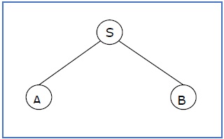
If S → x₁x₂ …… x_n is a production rule in a CFG, then the parse tree / derivation tree will be as follows −

There are two different approaches to draw a derivation tree −

Top-down Approach −

Starts with the starting symbol S
Goes down to tree leaves using productions

Bottom-up Approach −

Starts from tree leaves
Proceeds upward to the root which is the starting symbol S

Derivation or Yield of a Tree

The derivation or the yield of a parse tree is the final string obtained by concatenating the labels of the leaves of the tree from left to right, ignoring the Nulls. However, if all the leaves are Null, derivation is Null.

Example

Let a CFG {N,T,P,S} be

N = {S}, T = {a, b}, Starting symbol = S, P = S → SS | aSb | ε

One derivation from the above CFG is “abaabb”

S → SS → aSbS → abS → abaSb → abaaSbb → abaabb

Sentential Form and Partial Derivation Tree

A partial derivation tree is a sub-tree of a derivation tree/parse tree such that either all of its children are in the sub-tree or none of them are in the sub-tree.

Example

If in any CFG the productions are −

S → AB, A → aaA | ε, B → Bb| ε

the partial derivation tree can be the following −

If a partial derivation tree contains the root S, it is called a sentential form. The above sub-tree is also in sentential form.

Leftmost and Rightmost Derivation of a String

Leftmost derivation − A leftmost derivation is obtained by applying production to the leftmost variable in each step.
Rightmost derivation − A rightmost derivation is obtained by applying production to the rightmost variable in each step.

Example

Let any set of production rules in a CFG be

X → X+X | X*X |X| a

over an alphabet {a}.

The leftmost derivation for the string "a+a*a" may be −

X → X+X → a+X → a + X*X → a+a*X → a+a*a

उपरोक्त स्ट्रिंग की स्टेपवाइज व्युत्पत्ति नीचे दी गई है -

उपरोक्त स्ट्रिंग के लिए सबसे सही व्युत्पत्ति "a+a*a" हो सकता है -

एक्स → एक्स * एक्स → एक्स * ए → एक्स + एक्स * ए → एक्स + ए * ए → ए + ए * ए

उपरोक्त स्ट्रिंग की स्टेपवाइज व्युत्पत्ति नीचे दी गई है -

बाएँ और दाएँ पुनरावर्ती व्याकरण

एक संदर्भ-मुक्त व्याकरण में G, अगर फार्म में उत्पादन होता है X → Xa कहाँ पे X एक गैर-टर्मिनल है और ‘a’ टर्मिनलों की एक स्ट्रिंग है, इसे ए कहा जाता है left recursive production। वाम पुनरावर्ती उत्पादन वाले व्याकरण को a कहा जाता हैleft recursive grammar।

और अगर एक संदर्भ-मुक्त व्याकरण में G, अगर वहाँ एक उत्पादन के रूप में है X → aX कहाँ पे X एक गैर-टर्मिनल है और ‘a’ टर्मिनलों की एक स्ट्रिंग है, इसे ए कहा जाता है right recursive production। एक सही पुनरावर्ती उत्पादन वाले व्याकरण को कहा जाता हैright recursive grammar।

यदि एक संदर्भ मुक्त व्याकरण G कुछ स्ट्रिंग के लिए एक से अधिक व्युत्पन्न पेड़ है w ∈ L(G), यह एक कहा जाता है ambiguous grammar। उस व्याकरण से उत्पन्न कुछ स्ट्रिंग के लिए कई दाएं-बाएं या सबसे अधिक व्युत्पन्न मौजूद हैं।

मुसीबत

जाँच करें कि क्या उत्पादन नियमों के साथ व्याकरण जी -

X → X + X | X * X | X | ए

अस्पष्ट है या नहीं।

उपाय

चलो स्ट्रिंग "एक ए + एक" के लिए व्युत्पन्न पेड़ का पता लगाएं। इसकी दो सबसे बाईं व्युत्पन्नियाँ हैं।

Derivation 1- एक्स → एक्स + एक्स → ए + एक्स → ए + एक्स * एक्स → ए + ए * एक्स → ए + ए * ए

Parse tree 1 -

Derivation 2- एक्स → एक्स * एक्स * एक्स → एक्स + एक्स * एक्स → ए + एक्स * एक्स → ए + ए * एक्स → ए + ए * ए

Parse tree 2 -

चूँकि एकल स्ट्रिंग "a + a * a", व्याकरण के लिए दो पार्स पेड़ हैं G अस्पष्ट है।

प्रसंग-मुक्त भाषाएँ हैं closed के तहत -

Union
Concatenation
क्लेन स्टार ऑपरेशन

संघ

बता दें कि L ₁ और L ₂ दो संदर्भ मुक्त भाषा हैं। फिर एल ₁ L एल ₂ भी संदर्भ मुक्त है।

उदाहरण

L ₁ = {a ⁿ b ⁿ , n> 0} करें। पत्राचार व्याकरण G ₁ में P: S1 → AAb | ab होगा

L ₂ = {c ^m d ^m , m। 0}। पत्राचार व्याकरण G ₂ में P: S2 → cBb होगा | ε

L ₁ और L ₂ का संघ , L = L ₁ { L ₂ = {a ⁿ b ⁿ } ∪ {c ^m d ^m }

इसी व्याकरण G में अतिरिक्त उत्पादन S → S1 होगा एस 2

कड़ी

यदि L ₁ और L ₂ संदर्भ मुक्त भाषाएं हैं, तो L ₁ L ₂ भी संदर्भ मुक्त है।

उदाहरण

भाषाओं का संघ L ₁ और L ₂ , L = L ₁ L ₂ = {a ⁿ b ⁿ c ^m d ^m }

इसी व्याकरण G में अतिरिक्त उत्पादन S → S1 S2 होगा

क्लेने स्टार

यदि L एक संदर्भ मुक्त भाषा है, तो L * भी संदर्भ मुक्त है।

उदाहरण

L = {a ⁿ b ⁿ , n। 0}। पत्राचार व्याकरण G में P: S → AAb | ε

क्लेन स्टार एल ₁ = {ए ^एन बी ^एन } *

इसी व्याकरण जी ₁ अतिरिक्त प्रस्तुतियों एस 1 → होगा एसएस ₁ | ε

प्रसंग-मुक्त भाषाएँ हैं not closed के तहत -

Intersection - यदि L1 और L2 संदर्भ मुक्त भाषा हैं, तो L1 is L2 आवश्यक रूप से संदर्भ मुक्त नहीं है।
Intersection with Regular Language - यदि L1 एक नियमित भाषा है और L2 एक संदर्भ मुक्त भाषा है, तो L1 1 L2 एक संदर्भ मुक्त भाषा है।
Complement - यदि L1 एक संदर्भ मुक्त भाषा है, तो L1 'संदर्भ मुक्त नहीं हो सकता है।

सीएफजी में, ऐसा हो सकता है कि स्ट्रिंग्स के व्युत्पन्न के लिए सभी उत्पादन नियमों और प्रतीकों की आवश्यकता नहीं है। इसके अलावा, कुछ अशक्त प्रोडक्शंस और यूनिट प्रोडक्शंस हो सकते हैं। इन प्रस्तुतियों और प्रतीकों का उन्मूलन कहा जाता हैsimplification of CFGs। सरलीकरण अनिवार्य रूप से निम्नलिखित चरणों में शामिल है -

सीएफजी की कमी
यूनिट प्रोडक्शंस को हटाना
अशक्त निर्माण हटाना

सीएफजी की कमी

CFG दो चरणों में कम हो जाते हैं -

Phase 1 - एक समान व्याकरण की व्युत्पत्ति, G’, सीएफजी से, G, ऐसा है कि प्रत्येक चर कुछ टर्मिनल स्ट्रिंग प्राप्त करता है।

Derivation Procedure -

चरण 1 - सभी प्रतीकों को शामिल करें, W₁, कि कुछ टर्मिनल प्राप्त करें और आरंभ करें i=1।

चरण 2 - सभी प्रतीकों को शामिल करें, W_i+1, कि व्युत्पन्न W_i।

चरण 3 - वृद्धि i और चरण 2 को दोहराएं, जब तक W_i+1 = W_i।

चरण 4 - उन सभी उत्पादन नियमों को शामिल करें जिनके पास है W_i इस में।

Phase 2 - एक समान व्याकरण की व्युत्पत्ति, G”, सीएफजी से, G’, ऐसा है कि प्रत्येक प्रतीक एक भावुक रूप में प्रकट होता है।

Derivation Procedure -

चरण 1 - प्रारंभ प्रतीक को शामिल करें Y₁ और इनिशियलाइज़ करें i = 1।

चरण 2 - सभी प्रतीकों को शामिल करें, Y_i+1, कि से प्राप्त किया जा सकता है Y_i और लागू किए गए सभी उत्पादन नियमों को शामिल करें।

चरण 3 - वृद्धि i और चरण 2 को दोहराएं, जब तक Y_i+1 = Y_i।

मुसीबत

उत्पादन नियम वाले व्याकरण G के बराबर एक घटा हुआ व्याकरण ज्ञात करें, P: S → AC | बी, ए → ए, सी → सी | बीसी, ई → एए | इ

उपाय

Phase 1 -

टी = {ए, सी, ई}

डब्ल्यू ₁ = {ए, सी, ई} नियमों से ए → ए, सी → सी और ई → एए

W ₂ = {A, C, E} U {S} नियम S → AC से

डब्ल्यू ₃ = {ए, सी, ई, एस} यू,

डब्ल्यू ₂ = डब्ल्यू _{3 के} बाद से , हम जी 'को प्राप्त कर सकते हैं -

जी '= {{ए, सी, ई, एस}, {ए, सी, ई}, पी, {एस}}

जहाँ P: S → AC, A →, C → c, E → AA | इ

Phase 2 -

Y ₁ = {S}

Y ₂ = {S, A, C} नियम S → AC से

वाई ₃ = {एस, ए, सी, ए, सी} नियमों से ए → ए और सी → सी

वाई ₄ = {एस, ए, सी, ए, सी}

Y ₃ = Y _{4 के} बाद से , हम G को प्राप्त कर सकते हैं -

जी ”= {{ए, सी, एस}, {ए, सी}, पी, {एस}}

जहाँ P: S → AC, A → A, C → c

यूनिट प्रोडक्शंस को हटाना

ए → बी के रूप में कोई भी उत्पादन नियम जहां ए, बी terminal नॉन-टर्मिनल कहा जाता है unit production.।

निष्कासन प्रक्रिया -

Step 1 - दूर करना A → B, उत्पादन जोड़ें A → x जब भी व्याकरण नियम के अनुसार B → xव्याकरण में होता है। [x ∈ टर्मिनल, x अशक्त हो सकता है]

Step 2 - हटाएँ A → B व्याकरण से।

Step 3 - चरण 1 से दोहराएँ जब तक सभी इकाई प्रस्तुतियों को हटा दिया जाता है।

Problem

निम्नलिखित से इकाई उत्पादन निकालें -

S → XY, X → a, Y → Z | बी, जेड → एम, एम → एन, एन → ए

Solution -

व्याकरण में 3 इकाई निर्माण हैं -

वाई → जेड, जेड → एम, और एम → एन

At first, we will remove M → N.

N → a के रूप में, हम M → a जोड़ते हैं, और M → N को हटा दिया जाता है।

उत्पादन सेट बन जाता है

S → XY, X → a, Y → Z | बी, जेड → एम, एम → ए, एन → ए

Now we will remove Z → M.

M → a के रूप में, हम Z → a जोड़ते हैं, और Z → M को हटा दिया जाता है।

उत्पादन सेट बन जाता है

S → XY, X → a, Y → Z | बी, जेड → ए, एम → ए, एन → ए

Now we will remove Y → Z.

Z → a के रूप में, हम Y → a जोड़ते हैं, और Y → Z हटा दिया जाता है।

उत्पादन सेट बन जाता है

S → XY, X → a, Y → a | बी, जेड → ए, एम → ए, एन → ए

अब Z, M और N अप्राप्य हैं, इसलिए हम उन्हें हटा सकते हैं।

अंतिम CFG इकाई उत्पादन मुक्त है -

S → XY, X → a, Y → a | ख

अशक्त निर्माण हटाना

सीएफजी में, एक गैर-टर्मिनल प्रतीक ‘A’ उत्पादन होने पर अशक्त चर है A → ε या एक व्युत्पत्ति है जो शुरू होती है A और अंत में समाप्त होता है

......: ए → .......… → ......

निष्कासन प्रक्रिया

Step 1 - अशक्त गैर-टर्मिनल वैरिएबल का पता लगाएं जो able प्राप्त करते हैं।

Step 2 - प्रत्येक उत्पादन के लिए A → a, सभी प्रस्तुतियों का निर्माण A → x कहाँ पे x से प्राप्त किया जाता है ‘a’ चरण 1 से एक या कई गैर-टर्मिनलों को हटाकर।

Step 3 - चरण 2 और हटाने के परिणाम के साथ मूल प्रस्तुतियों को मिलाएं ε - productions।

Problem

निम्नलिखित से शून्य उत्पादन निकालें -

एस → एएसए | aB | बी, ए → बी, बी → बी | ∈

Solution -

दो अशक्त चर हैं - A तथा B

At first, we will remove B → ε.

निकालने के बाद B → ε, उत्पादन सेट बन जाता है -

एस → एएसए | aB | बी | ए, ए, बी | बी | & एप्सिलॉन, बी → बी

Now we will remove A → ε.

निकालने के बाद A → ε, उत्पादन सेट बन जाता है -

एस → एएसए | aB | बी | ए | SA | के रूप में | एस, ए → बी | बी, बी → बी

यह शून्य संक्रमण के बिना अंतिम उत्पादन सेट है।

यदि प्रोडक्शंस निम्नलिखित रूपों में हैं तो एक सीएफजी चॉम्स्की नॉर्मल फॉर्म में है -

ए → ए
A → ई.पू.
एस → ε

जहां A, B और C गैर-टर्मिनल हैं और a टर्मिनल है।

चॉम्स्की सामान्य रूप में परिवर्तित करने के लिए एल्गोरिथम -

Step 1 - अगर स्टार्ट सिंबल S कुछ दाईं ओर होता है, एक नया प्रारंभ प्रतीक बनाएँ S’ और एक नया उत्पादन S’→ S।

Step 2- अशक्त प्रस्तुतियों को हटा दें। (पहले चर्चा की गई नल उत्पादन हटाने एल्गोरिथ्म का उपयोग करना)

Step 3- यूनिट प्रोडक्शंस निकालें। (यूनिट उत्पादन हटाने एल्गोरिथ्म का उपयोग पहले चर्चा की)

Step 4 - प्रत्येक उत्पादन बदलें A → B₁…B_n कहाँ पे n > 2 साथ में A → B₁C कहाँ पे C → B₂ …B_n। दाईं ओर दो या दो से अधिक प्रतीकों वाली सभी प्रस्तुतियों के लिए इस चरण को दोहराएं।

Step 5 - यदि किसी भी उत्पादन का सही पक्ष फॉर्म में है A → aB जहां एक टर्मिनल है और A, B गैर-टर्मिनल हैं, फिर उत्पादन द्वारा प्रतिस्थापित किया जाता है A → XB तथा X → a। प्रत्येक उत्पादन के लिए इस चरण को दोहराएं जो फॉर्म में हैA → aB।

मुसीबत

निम्नलिखित CFG को CNF में परिवर्तित करें

एस → एएसए | ए बी, ए → बी | एस, बी → बी | ε

उपाय

(1) जबसे S RHS में प्रकट होता है, हम एक नया राज्य जोड़ते हैं S₀ तथा S₀→S उत्पादन सेट में जोड़ा जाता है और यह बन जाता है -

एस ₀ → एस, एस → एएसए | ए बी, ए → बी | एस, बी → बी | ∈

(2) अब हम अशक्त प्रस्तुतियों को हटा देंगे -

बी → A और ए → A

बी → ε को हटाने के बाद, उत्पादन सेट बन जाता है -

एस ₀ → एस, एस → एएसए | aB | ए, ए → बी | एस | B, बी → बी

A → ∈ को हटाने के बाद, उत्पादन सेट बन जाता है -

एस ₀ → एस, एस → एएसए | aB | ए | के रूप में | SA | एस, ए → बी | एस, बी → बी

(3) अब हम यूनिट प्रोडक्शंस को हटा देंगे।

S → S को हटाने के बाद, उत्पादन सेट बन जाता है -

S ₀ → S को हटाने के बाद , उत्पादन सेट बन जाता है -

एस ₀ → एएसए | aB | ए | के रूप में | एसए, एस → एएसए | aB | ए | के रूप में | एसए

ए → बी | एस, बी → बी

A → B निकालने के बाद, उत्पादन सेट बन जाता है -

एस ₀ → एएसए | aB | ए | के रूप में | एसए, एस → एएसए | aB | ए | के रूप में | एसए

ए → एस | ख

बी → बी

ए → एस को हटाने के बाद, उत्पादन सेट बन जाता है -

एस ₀ → एएसए | aB | ए | के रूप में | एसए, एस → एएसए | aB | ए | के रूप में | एसए

A → b | ASA | aB | ए | के रूप में | एसए, बी → बी

(4) अब हम आरएचएस में दो से अधिक वेरिएबल्स का पता लगाएंगे

यहाँ, S ₀ → ASA, S → ASA, A → ASA RHS में दो गैर-टर्मिनलों का उल्लंघन करता है

इसलिए हम निम्नलिखित अंतिम उत्पादन सेट प्राप्त करने के लिए चरण 4 और चरण 5 लागू करेंगे जो CNF में है -

S ₀ → AX | aB | ए | के रूप में | एसए

S → AX | aB | ए | के रूप में | एसए

A → b | AX | aB | ए | के रूप में | एसए

बी → बी

एक्स → एसए

(5)हमें प्रोडक्शंस S ₀ → aB, S → aB, A → aB बदलना होगा

और अंतिम उत्पादन सेट बन जाता है -

S ₀ → AX | YB | ए | के रूप में | एसए

S → AX | YB | ए | के रूप में | एसए

A → b A → b | AX | YB | ए | के रूप में | एसए

बी → बी

एक्स → एसए

Y → a

यदि प्रोडक्शंस निम्नलिखित रूपों में हैं तो एक सीएफजी ग्रीबाच नॉर्मल फॉर्म में है -

ए → बी

A → bD ₁ ... D _n

एस → ε

जहाँ A, D ₁ , ...., D _n गैर-टर्मिनल हैं और b एक टर्मिनल है।

एक CFG को ग्रीबच नॉर्मल फॉर्म में बदलने के लिए एल्गोरिदम

Step 4 - सभी प्रत्यक्ष और अप्रत्यक्ष वाम-पुनरावृत्ति को हटा दें।

Step 5 - इसे GNF के उचित रूप में परिवर्तित करने के लिए प्रस्तुतियों का उचित प्रतिस्थापन करें।

मुसीबत

निम्नलिखित CFG को CNF में परिवर्तित करें

S → XY | Xn | पी

एक्स → एमएक्स | म

Y → Xn | हे

उपाय

यहाँ, Sकिसी भी उत्पादन के दाईं ओर दिखाई नहीं देता है और उत्पादन नियम सेट में कोई इकाई या अशक्त प्रोडक्शंस नहीं हैं। तो, हम चरण 1 को चरण 3 पर छोड़ सकते हैं।

Step 4

अब बदलने के बाद

X इन S → XY | Xo | पी

साथ में

एमएक्स | म

हमने प्राप्त किया

एस → एमएक्सवाई | एमवाय | mXo | मो | पी

और बदलने के बाद

X in Y → X _n | हे

के दाईं ओर

एक्स → एमएक्स | म

हमने प्राप्त किया

Y → mXn | एमएन | ओ

दो नए निर्माण O → o और P → p को उत्पादन सेट में जोड़ा जाता है और फिर हम निम्नलिखित के रूप में अंतिम GNF में आए -

एस → एमएक्सवाई | एमवाय | एमएक्ससी | mC | पी

एक्स → एमएक्स | म

Y → mXD | mD | हे

ओ → ओ

पी → पी

लेम्मा

अगर L एक संदर्भ-मुक्त भाषा है, एक पंपिंग लंबाई है p ऐसे कि कोई भी तार w ∈ L लंबाई की ≥ p के रूप में लिखा जा सकता है w = uvxyz, कहाँ पे vy ≠ ε, |vxy| ≤ p, और सभी के लिए i ≥ 0, uvⁱxyⁱz ∈ L।

पम्पिंग लेम्मा के अनुप्रयोग

पम्पिंग लेम्मा का उपयोग यह जांचने के लिए किया जाता है कि कोई व्याकरण संदर्भ मुक्त है या नहीं। आइए एक उदाहरण लेते हैं और दिखाते हैं कि यह कैसे जांचा जाता है।

मुसीबत

पता करें कि क्या भाषा L = {xⁿyⁿzⁿ | n ≥ 1} संदर्भ मुक्त है या नहीं।

उपाय

लश्कर Lसंदर्भ मुक्त है। फिर,L पम्पिंग लेम्मा को संतुष्ट करना चाहिए।

सबसे पहले, एक नंबर चुनें nपम्पिंग लेम्मा। फिर, 0 ⁿ 1 ⁿ 2 ^{n के} रूप में z लें ।

टूटना z जांच uvwxy, कहाँ पे

|vwx| ≤ n and vx ≠ ε.

इसलिये vwx0 और 2s दोनों को शामिल नहीं कर सकता, क्योंकि अंतिम 0 और पहले 2 अलग-अलग हैं (n + 1) स्थिति। दो मामले हैं -

Case 1 - vwxकोई 2s है। फिरvxकेवल 0s और 1s है। फिरuwy, जो अंदर होना होगा L, है n 2s, लेकिन से कम n 0 या 1 एस।

Case 2 - vwx कोई 0s है।

यहां विरोधाभास होता है।

इसलिये, L एक संदर्भ-मुक्त भाषा नहीं है।

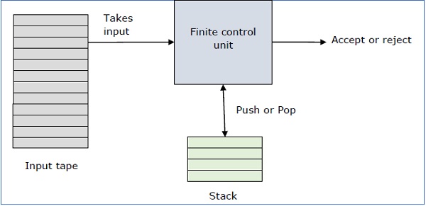
पीडीए की मूल संरचना

एक पुशडाउन ऑटोमेटन इसी तरह से एक संदर्भ-मुक्त व्याकरण को लागू करने का एक तरीका है, जिसे हम एक नियमित व्याकरण के लिए DFA डिज़ाइन करते हैं। DFA जानकारी की एक सीमित मात्रा को याद रख सकता है, लेकिन एक पीडीए जानकारी की अनंत मात्रा को याद रख सकता है।

मूल रूप से एक पुशडाउन ऑटोमेटन है -

"Finite state machine" + "a stack"

एक पुशडाउन ऑटोमेटन के तीन घटक हैं -

एक इनपुट टेप,
एक नियंत्रण इकाई, और
अनंत आकार के साथ एक ढेर।

स्टैक हेड स्टैक के शीर्ष प्रतीक को स्कैन करता है।

एक स्टैक दो ऑपरेशन करता है -

Push - शीर्ष पर एक नया प्रतीक जोड़ा जाता है।
Pop - शीर्ष प्रतीक को पढ़ा और हटा दिया गया है।

एक पीडीए एक इनपुट प्रतीक को पढ़ या नहीं सकता है, लेकिन इसे हर संक्रमण में स्टैक के शीर्ष को पढ़ना होगा।

एक पीडीए को औपचारिक रूप से 7-ट्यूपल (Q, form, S, δ, q ₀ , I, F) के रूप में वर्णित किया जा सकता है -

Q राज्यों की परिमित संख्या है
∑ इनपुट वर्णमाला है
S स्टैक प्रतीक है
δ संक्रमण समारोह है: Q × (∑ transition {)}) × S × Q × S *
q₀प्रारंभिक अवस्था है (q ₀ ∈ Q)
I प्रारंभिक स्टैक शीर्ष प्रतीक है (I) S)
F राज्यों को स्वीकार करने का एक सेट है (F set Q)

निम्नलिखित चित्र एक पीडीए में राज्य क्यू ₁ से राज्य क्यू ₂ तक एक संक्रमण को दर्शाता है , जिसे ए, बी → सी - के रूप में लेबल किया गया है।

राज्य में इसका मतलब है q₁, अगर हम एक इनपुट स्ट्रिंग का सामना करते हैं ‘a’ और स्टैक का शीर्ष प्रतीक है ‘b’, फिर हम पॉप ‘b’, धक्का दें ‘c’ ढेर के ऊपर और राज्य के लिए आगे बढ़ें q₂।

पीडीए से संबंधित शब्दावली

तात्कालिक विवरण

पीडीए का तात्कालिक विवरण (आईडी) एक ट्रिपल (क्यू, डब्ल्यू, एस) द्वारा दर्शाया जाता है

q राज्य है
w गैर-इनपुट इनपुट है
s स्टैक सामग्री है

घूमने-फिरने की सूचना

"टर्नस्टाइल" नोटेशन का उपयोग आईडी के जोड़े को जोड़ने के लिए किया जाता है जो पीडीए के एक या कई चालों का प्रतिनिधित्व करते हैं। संक्रमण की प्रक्रिया को टर्नस्टाइल प्रतीक "den" द्वारा निरूपित किया जाता है।

एक पीडीए (क्यू, ∑, एस, q, क्यू ₀ , आई, एफ) पर विचार करें। एक संक्रमण को गणितीय रूप से निम्नलिखित घूमने वाले अंकन द्वारा दर्शाया जा सकता है -

(p, aw, Tβ) ⊢ (q, w, αb)

इसका तात्पर्य यह है कि राज्य से संक्रमण लेते समय p कहना q, इनपुट प्रतीक ‘a’ भस्म हो गया है, और ढेर के ऊपर ‘T’ एक नई स्ट्रिंग द्वारा प्रतिस्थापित किया जाता है ‘α’।

Note - यदि हम पीडीए के शून्य या अधिक चाल चाहते हैं, तो हमें इसके लिए प्रतीक (want *) का उपयोग करना होगा।

पीडीए स्वीकार्यता को परिभाषित करने के दो अलग-अलग तरीके हैं।

अंतिम राज्य की स्वीकार्यता

अंतिम राज्य की स्वीकार्यता में, एक पीडीए एक स्ट्रिंग को स्वीकार करता है, जब पूरे स्ट्रिंग को पढ़ने के बाद, पीडीए एक अंतिम स्थिति में है। प्रारंभिक अवस्था से, हम ऐसी चालें बना सकते हैं जो अंतिम अवस्था में किसी भी स्टैक मान के साथ समाप्त होती हैं। जब तक हम अंतिम स्थिति में होते हैं तब तक ढेर के मूल्य अप्रासंगिक होते हैं।

एक पीडीए (Q, ∑, S, q, q ₀ , I, F) के लिए, अंतिम राज्यों F के सेट द्वारा स्वीकृत भाषा है -

एल (पीडीए) = {w | (q ₀ , w, I) (* (q,,, x), q} F}

किसी भी इनपुट स्टैक स्ट्रिंग के लिए x।

खाली स्टैक स्वीकार्यता

यहां एक पीडीए एक स्ट्रिंग को स्वीकार करता है, जब पूरे स्ट्रिंग को पढ़ने के बाद, पीडीए ने अपने स्टैक को खाली कर दिया है।

एक पीडीए (Q, S, S, q, q ₀ , I, F) के लिए, खाली स्टैक द्वारा स्वीकार की गई भाषा -

एल (पीडीए) = {w | (q ₀ , w, I) ⊢ * (q,,,,), q} Q}

उदाहरण

एक पीडीए का निर्माण करता है जो स्वीकार करता है L = {0ⁿ 1ⁿ | n ≥ 0}

उपाय

यह भाषा L = {ε, 01, 0011, 000111, …………………………} स्वीकार करती है।

यहाँ, इस उदाहरण में, की संख्या ‘a’ तथा ‘b’ एक ही होना है।

प्रारंभ में हमने एक विशेष प्रतीक रखा ‘$’ खाली ढेर में।
फिर राज्य में q₂, अगर हमारे पास इनपुट 0 है और शीर्ष अशक्त है, तो हम 0 को स्टैक में धकेल देते हैं। यह पुनरावृति हो सकती है। और अगर हम 1 इनपुट का सामना करते हैं और शीर्ष 0 है, तो हम इस 0 को पॉप करते हैं।
फिर राज्य में q₃, अगर हम 1 इनपुट का सामना करते हैं और शीर्ष 0 है, तो हम इसे 0. पॉप करते हैं। यह भी पुनरावृति हो सकता है। और अगर हम 1 इनपुट का सामना करते हैं और शीर्ष 0 है, तो हम शीर्ष तत्व को पॉप करते हैं।
यदि स्टैक के शीर्ष पर विशेष प्रतीक '$' अंकित है, तो यह पॉप आउट हो जाता है और अंत में इसे स्वीकार करने की स्थिति q _{4 हो जाती है} ।

उदाहरण

एक पीडीए है कि एल स्वीकार करता है का निर्माण = {ww ^आर | w = (a + b) *}

Solution

प्रारंभ में हम खाली स्टैक में एक विशेष प्रतीक '$' डालते हैं। राज्य मेंq₂, को wपढ़ा जा रहा है। राज्य मेंq₃प्रत्येक 0 या 1 को पॉप अप किया जाता है जब वह इनपुट से मेल खाता है। यदि कोई अन्य इनपुट दिया जाता है, तो पीडीए मृत अवस्था में चला जाएगा। जब हम उस विशेष प्रतीक '$' पर पहुँचते हैं, तो हम स्वीकार करने की स्थिति में जाते हैंq₄।

यदि कोई व्याकरण G संदर्भ-मुक्त है, हम एक समतुल्य nondeterministic PDA का निर्माण कर सकते हैं, जो उस भाषा को स्वीकार करता है जो संदर्भ-मुक्त व्याकरण द्वारा निर्मित होती है G। व्याकरण के लिए एक पार्सर बनाया जा सकता हैG।

इसके अलावा यदि P एक पुशडाउन ऑटोमेटन है, जहां एक समान संदर्भ-मुक्त व्याकरण जी का निर्माण किया जा सकता है

L(G) = L(P)

अगले दो विषयों में, हम चर्चा करेंगे कि पीडीए से सीएफजी और इसके विपरीत कैसे परिवर्तित किया जाए।

पीडीए को दिए गए CFG के अनुरूप खोजने के लिए एल्गोरिथम

Input - एक सीएफजी, जी = (वी, टी, पी, एस)

Output- समतुल्य पीडीए, पी = (क्यू, S, एस, q, क्यू ₀ , आई, एफ)

Step 1 - CFG की प्रस्तुतियों को GNF में बदलें।

Step 2 - पीडीए में केवल एक राज्य {q} होगा।

Step 3 - सीएफजी का स्टार्ट सिंबल पीडीए में स्टार्ट सिंबल होगा।

Step 4 - सीएफजी के सभी गैर-टर्मिनल पीडीए के स्टैक प्रतीक होंगे और सीएफजी के सभी टर्मिनल पीडीए के इनपुट प्रतीक होंगे।

Step 5 - फार्म में प्रत्येक उत्पादन के लिए A → aX जहां एक टर्मिनल है और A, X टर्मिनल और गैर-टर्मिनलों का संयोजन है, एक संक्रमण बनाते हैं δ (q, a, A)।

मुसीबत

निम्नलिखित CFG से पीडीए का निर्माण करें।

G = ({S, X}, {a, b}, P, S)

प्रोडक्शंस कहाँ हैं -

S → XS | ε , A → aXb | Ab | ab

उपाय

समकक्ष PDA,

P = ({q}, {a, b}, {a, b, X, S}, δ, q, S)

कहाँ δ -

ε (q, ε, S) = {(q, XS), (q, q)}

ε (q, ε, X) = {(q, aXb), (q, Xb), (q, ab)}

a (q, a, a) = {(q, a)}

1 (q, 1, 1) = {(q, 1)}

दिए गए पीडीए के अनुरूप सीएफजी को खोजने के लिए एल्गोरिदम

Input - एक सीएफजी, जी = (वी, टी, पी, एस)

Output- समतुल्य पीडीए, पी = (क्यू, S, एस , A , क्यू ₀ , आई, एफ) जैसे कि व्याकरण जी के गैर-टर्मिनल {एक्स _{डब्ल्यूएक्स} | w, x, Q} और प्रारंभ स्थिति A _{q0, F होगी} ।

Step 1- प्रत्येक w के लिए, x, y, z m Q, m a S और a, b ∑ x, यदि a (w, a, ε) समाहित है (y, m) और (z, b, m) समाहित है (x, w) ε), व्याकरण G में उत्पादन नियम X _wx → एक X _yz b जोड़ें।

Step 2- प्रत्येक w, x, y, z add Q के लिए, व्याकरण जी में उत्पादन नियम X _wx → X _wy X _{yx जोड़ें} ।

Step 3- w For Q के लिए, व्याकरण G में उत्पादन नियम X _ww → ∈ जोड़ें ।

पार्सिंग का उपयोग एक व्याकरण के उत्पादन नियमों का उपयोग करके एक स्ट्रिंग प्राप्त करने के लिए किया जाता है। यह एक स्ट्रिंग की स्वीकार्यता की जांच करने के लिए उपयोग किया जाता है। कंपाइलर का उपयोग यह जांचने के लिए किया जाता है कि कोई स्ट्रिंग वाक्यविन्यास रूप से सही है या नहीं। एक पार्सर इनपुट लेता है और एक पार्स ट्री बनाता है।

एक पार्सर दो प्रकार का हो सकता है -

Top-Down Parser - टॉप-डाउन पार्सिंग शुरू-प्रतीक के साथ ऊपर से शुरू होती है और एक पार्स ट्री का उपयोग करके एक स्ट्रिंग प्राप्त करती है।
Bottom-Up Parser - बॉटम-अप पार्सिंग स्ट्रिंग के साथ नीचे से शुरू होती है और पार्स ट्री का उपयोग करके स्टार्ट सिंबल पर आती है।

टॉप-डाउन पार्सर का डिज़ाइन

टॉप-डाउन पार्सिंग के लिए, एक पीडीए में निम्नलिखित चार प्रकार के संक्रमण होते हैं -

स्टैक के शीर्ष पर उत्पादन के बाएं हाथ पर गैर-टर्मिनल को पॉप करें और उसके दाहिने हाथ की तरफ स्ट्रिंग को धक्का दें।
यदि स्टैक का शीर्ष प्रतीक पढ़ा जा रहा इनपुट प्रतीक से मेल खाता है, तो इसे पॉप करें।
स्टैक में प्रारंभ प्रतीक 'S' को दबाएं।
यदि इनपुट स्ट्रिंग पूरी तरह से पढ़ी गई है और स्टैक खाली है, तो अंतिम स्थिति 'एफ' पर जाएं।

उदाहरण

निम्नलिखित उत्पादन नियमों के साथ व्याकरण G के लिए अभिव्यक्ति "x + y * z" के लिए एक टॉप-डाउन पार्सर डिज़ाइन करें -

P: S → S + X | एक्स, एक्स → एक्स * वाई | वाई, वाई → (एस) | ईद

Solution

यदि PDA है (Q, (, S, q, q ₀ , I, F), तो ऊपर-नीचे पार्स है -

(x + y * z, I) ⊢ (x + y * z, SI) z (x + y * z, S + XI) ⊢ (x + y * z, X + XI)

Y (x + y * z, Y + XI) x (x + y * z, x + XI) y (+ y * z, + XI) ⊢ (y * z, XI)

, (Y * z, X * YI) y (y * z, y * YI) ⊢ (* z, * YI) z (z, YI) z (z, zI) ⊢ (ε, I)

एक बॉटम-अप पार्सर का डिज़ाइन

नीचे-अप पार्सिंग के लिए, एक पीडीए में निम्नलिखित चार प्रकार के संक्रमण होते हैं -

स्टैक में वर्तमान इनपुट प्रतीक को पुश करें।
स्टैक के शीर्ष पर किसी प्रोडक्शन के राइट-हैंड साइड को उसके लेफ्ट-हैंड साइड से बदलें।
यदि स्टैक तत्व का शीर्ष वर्तमान इनपुट प्रतीक के साथ मेल खाता है, तो इसे पॉप करें।
यदि इनपुट स्ट्रिंग पूरी तरह से पढ़ी जाती है और केवल तभी जब स्टार्ट सिंबल 'S' स्टैक में रहता है, तो इसे पॉप करें और अंतिम स्थिति 'F' पर जाएं।

उदाहरण

P: S → S + X | एक्स, एक्स → एक्स * वाई | वाई, वाई → (एस) | ईद

Solution

यदि PDA है (Q, (, S, (, q ₀ , I, F), तो नीचे-ऊपर पार्स है -

(x + y * z, I) ⊢ (+ y * z, xI) z (+ y * z, YI) z (+ y * z, XI) ⊢ (+ y * z, SI)

Z (y * z, + SI) ⊢ (* z, y + SI) z (* z, Y + SI) z (* z, X + SI) ⊢ (z, * X + SI)

Ε (⊢, z * X + SI) ε (Y, Y * X + SI) ε (SI, X + SI) ⊢ (ε, SI)

ट्यूरिंग मशीन एक स्वीकार करने वाला उपकरण है जो टाइप 0 व्याकरण द्वारा उत्पन्न भाषाओं (पुनरावर्ती असंख्य सेट) को स्वीकार करता है। इसका आविष्कार 1936 में एलन ट्यूरिंग ने किया था।

परिभाषा

ट्यूरिंग मशीन (टीएम) एक गणितीय मॉडल है जिसमें एक अनंत लंबाई की टेप होती है जो कोशिकाओं में विभाजित होती है जिस पर इनपुट दिया जाता है। इसमें एक सिर होता है जो इनपुट टेप को पढ़ता है। एक राज्य रजिस्टर ट्यूरिंग मशीन की स्थिति को संग्रहीत करता है। एक इनपुट प्रतीक को पढ़ने के बाद, इसे दूसरे प्रतीक से बदल दिया जाता है, इसकी आंतरिक स्थिति को बदल दिया जाता है, और यह एक कोशिका से दाएं या बाएं स्थानांतरित होता है। यदि TM अंतिम स्थिति में पहुंच जाता है, तो इनपुट स्ट्रिंग को स्वीकार कर लिया जाता है, अन्यथा अस्वीकार कर दिया जाता है।

एक टीएम को औपचारिक रूप से 7-ट्यूपल (क्यू, एक्स, δ, δ, q ₀ , B, F के रूप में वर्णित किया जा सकता है ) -

Q राज्यों का एक समुच्चय है
X टेप वर्णमाला है
∑ इनपुट वर्णमाला है
δएक संक्रमण समारोह है; X: Q × X → Q × X × {Left_shift, Right_shift}।
q₀ प्रारंभिक अवस्था है
B रिक्त प्रतीक है
F अंतिम राज्यों का सेट है

पिछले ऑटोमेटन के साथ तुलना

निम्न तालिका इस बात की तुलना करती है कि ट्यूरिंग मशीन, Finite Automaton और Pushdown Automaton से कैसे भिन्न है।

मशीन	स्टैक डेटा संरचना	नियतात्मक?
परिमित ऑटोमेटन	ना	हाँ
पुशडाउन ऑटोमेटन	पहले आउट में अंतिम (LIFO)	नहीं
ट्यूरिंग मशीन	अनंत टेप	हाँ

ट्यूरिंग मशीन का उदाहरण

ट्यूरिंग मशीन M = (Q, X, machine, q, q ₀ , B, F) के साथ

Q = {q ₀ , q ₁ , q ₂ , q _f }
X = {a, b}
1 = {1}
q ₀ = {q ₀ }
ब = खाली प्रतीक
F = {q _f }

by द्वारा दिया गया है -

टेप वर्णमाला प्रतीक	वर्तमान स्थिति 'q ₀ '	वर्तमान स्थिति 'q ₁ '	वर्तमान स्थिति 'q ₂ '
ए	_१ रक _१	१ लक _०	1 एल _एफ
ख	_१ लक _२	_१ रक _१	1 आर _एफ

यहां संक्रमण 1Rq _{1 का} अर्थ है कि लेखन प्रतीक 1 है, टेप सही चलता है, और अगला राज्य q _{1 है} । इसी तरह, संक्रमण 1Lq _{2 का} अर्थ है कि लेखन प्रतीक 1 है, टेप बाईं ओर चलता है, और अगला राज्य q _{2 है} ।

ट्यूरिंग मशीन का समय और स्थान जटिलता

ट्यूरिंग मशीन के लिए, समय जटिलता उस समय की संख्या को मापती है, जब टेप कुछ चालों की संख्या को मापता है जब मशीन को कुछ इनपुट प्रतीकों के लिए आरम्भ किया जाता है और अंतरिक्ष जटिलता लिखे गए टेप की कोशिकाओं की संख्या होती है।

समय जटिलता सभी उचित कार्य -

T(n) = O(n log n)

टीएम की अंतरिक्ष जटिलता -

S(n) = O(n)

यदि कोई इनपुट स्ट्रिंग w के लिए अंतिम स्थिति में प्रवेश करता है तो एक टीएम एक भाषा को स्वीकार करता है। यदि ट्यूरिंग मशीन द्वारा स्वीकार किया जाता है तो एक भाषा पुनरावर्ती रूप से टाइप करने योग्य (टाइप -0 व्याकरण से उत्पन्न) है।

एक टीएम एक भाषा का फैसला करता है अगर वह इसे स्वीकार करता है और किसी भी इनपुट के लिए अस्वीकार की स्थिति में प्रवेश करता है, तो भाषा में नहीं। यदि ट्यूरिंग मशीन द्वारा निर्णय लिया जाता है तो एक भाषा पुनरावर्ती है।

कुछ ऐसे मामले हो सकते हैं जहां एक टीएम बंद नहीं होता है। ऐसे टीएम भाषा को स्वीकार करते हैं, लेकिन यह इसे तय नहीं करता है।

ट्यूरिंग मशीन डिजाइन करना

ट्यूरिंग मशीन को डिजाइन करने के मूल दिशानिर्देशों को कुछ उदाहरणों की मदद से नीचे समझाया गया है।

उदाहरण 1

Α की विषम संख्या वाले सभी तारों को पहचानने के लिए एक TM डिज़ाइन करें।

Solution

ट्यूरिंग मशीन M निम्नलिखित चालों द्वारा निर्मित किया जा सकता है -

लश्कर q₁ प्रारंभिक अवस्था हो।
अगर M में है q₁; स्कैनिंग पर α, यह राज्य में प्रवेश करती हैq₂ और लिखता है B (खाली)।
अगर M में है q₂; स्कैनिंग पर α, यह राज्य में प्रवेश करती हैq₁ और लिखता है B (खाली)।
उपरोक्त चाल से, हम यह देख सकते हैं M राज्य में प्रवेश करता है q₁ अगर यह α's की एक समान संख्या को स्कैन करता है, और यह राज्य में प्रवेश करता है q₂अगर यह α की विषम संख्या को स्कैन करता है। इसलियेq₂ केवल स्वीकार करने वाला राज्य है।

इसलिये,

M = {{q ₁ , q ₂ }, {1}, {1, B}, {, q ₁ , B, { ₁ }}

where कहां दिया जाता है -

टेप वर्णमाला प्रतीक	वर्तमान स्थिति 'q ₁ '	वर्तमान स्थिति 'q ₂ '
α	ब्रिक _२	ब्रिक _१

उदाहरण 2

एक ट्यूरिंग मशीन डिज़ाइन करें जो एक बाइनरी नंबर का प्रतिनिधित्व करने वाले स्ट्रिंग को पढ़ता है और स्ट्रिंग में सभी प्रमुख 0 मिटा देता है। हालाँकि, यदि स्ट्रिंग में केवल 0 का समावेश है, तो यह एक 0 रखता है।

Solution

आइए हम मानते हैं कि इनपुट स्ट्रिंग को स्ट्रिंग के प्रत्येक छोर पर एक खाली प्रतीक, बी द्वारा समाप्त किया जाता है।

ट्यूरिंग मशीन, M, निम्नलिखित चालों द्वारा निर्मित किया जा सकता है -

लश्कर q₀ प्रारंभिक अवस्था हो।
अगर M में है q₀, 0 पढ़ने पर, यह सही चलता है, राज्य में प्रवेश करता है q₁ और मिटा देता है। 1 पढ़ने पर, यह राज्य में प्रवेश करता है q₂ और सही चलता है।
अगर M में है q₁, 0 पढ़ने पर, यह सही चलता है और 0 मिटाता है, अर्थात, यह B के द्वारा 0 की जगह लेता है। सबसे बाईं ओर पहुँचने पर, यह प्रवेश करता हैq₂और सही चलता है। यदि यह B तक पहुंचता है, यानी, स्ट्रिंग में केवल 0 का समावेश होता है, तो यह बाईं ओर चलती है और राज्य में प्रवेश करती हैq₃।
अगर M में है q₂, 0 या 1 पढ़ने पर, यह सही चलता है। बी तक पहुंचने पर, यह बाएं ओर बढ़ता है और राज्य में प्रवेश करता हैq₄। यह पुष्टि करता है कि स्ट्रिंग में केवल 0 और 1 का समावेश है।
अगर M में है q₃, यह B को 0 से बदल देता है, बाएं चलता है और अंतिम स्थिति में पहुंच जाता है q_f।
अगर M में है q₄, या तो 0 या 1 पढ़ने पर, यह बाईं ओर चलता है। स्ट्रिंग की शुरुआत तक पहुंचने पर, यानी, जब यह बी को पढ़ता है, तो यह अंतिम स्थिति तक पहुंचता हैq_f।

इसलिये,

M = {{q ₀ , q ₁ , q ₂ , q ₃ , q ₄ , q _f }, {0,1, B}, {1, B}, δ, q ₀ , B, {q _f }}

where कहां दिया जाता है -

टेप वर्णमाला प्रतीक	वर्तमान स्थिति 'q ₀ '	वर्तमान स्थिति 'q ₁ '	वर्तमान स्थिति 'q ₂ '	वर्तमान स्थिति 'q ₃ '	वर्तमान स्थिति 'q ₄ '
0	ब्रिक _१	ब्रिक _१	ओरक _२	-	ओलक _४
1	_१ रक _२	_१ रक _२	_१ रक _२	-	1Lq ₄
ख	ब्रिक _१	बीलक _३	ब्लक _४	ओलक _च	BRq _एफ

मल्टी-टेप ट्यूरिंग मशीनों में कई टेप होते हैं जहां प्रत्येक टेप को एक अलग सिर के साथ एक्सेस किया जाता है। प्रत्येक सिर दूसरे सिर से स्वतंत्र रूप से आगे बढ़ सकता है। प्रारंभ में इनपुट 1 टेप पर है और अन्य रिक्त हैं। पहले पर, पहले टेप पर इनपुट का कब्जा होता है और दूसरे टेप को खाली रखा जाता है। अगला, मशीन अपने सिर के नीचे लगातार प्रतीकों को पढ़ती है और टीएम प्रत्येक टेप पर एक प्रतीक प्रिंट करता है और अपने सिर को स्थानांतरित करता है।

एक मल्टी-टेप ट्यूरिंग मशीन को औपचारिक रूप से 6-ट्यूपल (Q, X, B,,, q ₀ , F) के रूप में वर्णित किया जा सकता है -

Q राज्यों का एक समुच्चय है
X टेप वर्णमाला है
B रिक्त प्रतीक है
δ जहां राज्यों और प्रतीकों पर एक संबंध है

X: Q × X ^k → Q × (X × {Left_shift, Right_shift, No_shift}) ^k

जहाँ ये है k टेपों की संख्या
q₀ प्रारंभिक अवस्था है
F अंतिम राज्यों का सेट है

Note - हर मल्टी-टेप ट्यूरिंग मशीन में एक सिंगल-टेप ट्यूरिंग मशीन होती है।

मल्टी-ट्रैक ट्यूरिंग मशीन, एक विशिष्ट प्रकार की मल्टी-टेप ट्यूरिंग मशीन, जिसमें कई ट्रैक होते हैं, लेकिन सिर्फ एक टेप हेड सभी पटरियों को पढ़ता और लिखता है। यहाँ, एक एकल टेप हेड से n प्रतीकों को पढ़ा जाता हैnएक कदम पर पटरियों। यह सामान्य एकल-ट्रैक सिंगल-टेप ट्यूरिंग मशीन की तरह पुनरावर्ती भाषाओं को स्वीकार करता है।

एक मल्टी-ट्रैक ट्यूरिंग मशीन को औपचारिक रूप से 6-ट्यूपल (Q, X, ∑,,, q ₀ , F) के रूप में वर्णित किया जा सकता है , जहां -

Q राज्यों का एक समुच्चय है
X टेप वर्णमाला है
∑ इनपुट वर्णमाला है
δ जहां राज्यों और प्रतीकों पर एक संबंध है

, (Q _i , [a ₁ , a ₂ , a, ₃ , ....) = = (Q _j , [b ₁ , b ₂ , b ₃ , ....], Left_shift या Right_shift)
q₀ is the initial state
F is the set of final states

Note − For every single-track Turing Machine S, there is an equivalent multi-track Turing Machine M such that L(S) = L(M).

In a Non-Deterministic Turing Machine, for every state and symbol, there are a group of actions the TM can have. So, here the transitions are not deterministic. The computation of a non-deterministic Turing Machine is a tree of configurations that can be reached from the start configuration.

An input is accepted if there is at least one node of the tree which is an accept configuration, otherwise it is not accepted. If all branches of the computational tree halt on all inputs, the non-deterministic Turing Machine is called a Decider and if for some input, all branches are rejected, the input is also rejected.

A non-deterministic Turing machine can be formally defined as a 6-tuple (Q, X, ∑, δ, q₀, B, F) where −

Q is a finite set of states
X is the tape alphabet
∑ is the input alphabet
δ is a transition function;

δ : Q × X → P(Q × X × {Left_shift, Right_shift}).
q₀ is the initial state
B is the blank symbol
F is the set of final states

A Turing Machine with a semi-infinite tape has a left end but no right end. The left end is limited with an end marker.

It is a two-track tape −

Upper track − It represents the cells to the right of the initial head position.
Lower track − It represents the cells to the left of the initial head position in reverse order.

The infinite length input string is initially written on the tape in contiguous tape cells.

The machine starts from the initial state q₀ and the head scans from the left end marker ‘End’. In each step, it reads the symbol on the tape under its head. It writes a new symbol on that tape cell and then it moves the head either into left or right one tape cell. A transition function determines the actions to be taken.

It has two special states called accept state and reject state. If at any point of time it enters into the accepted state, the input is accepted and if it enters into the reject state, the input is rejected by the TM. In some cases, it continues to run infinitely without being accepted or rejected for some certain input symbols.

Note − Turing machines with semi-infinite tape are equivalent to standard Turing machines.

A linear bounded automaton is a multi-track non-deterministic Turing machine with a tape of some bounded finite length.

Length = function (Length of the initial input string, constant c)

Here,

Memory information ≤ c × Input information

The computation is restricted to the constant bounded area. The input alphabet contains two special symbols which serve as left end markers and right end markers which mean the transitions neither move to the left of the left end marker nor to the right of the right end marker of the tape.

A linear bounded automaton can be defined as an 8-tuple (Q, X, ∑, q₀, ML, MR, δ, F) where −

Q is a finite set of states
X is the tape alphabet
∑ is the input alphabet
q₀ is the initial state
M_L is the left end marker
M_R is the right end marker where M_R ≠ M_L
δ is a transition function which maps each pair (state, tape symbol) to (state, tape symbol, Constant ‘c’) where c can be 0 or +1 or -1
F is the set of final states

A deterministic linear bounded automaton is always context-sensitive and the linear bounded automaton with empty language is undecidable..

A language is called Decidable or Recursive if there is a Turing machine which accepts and halts on every input string w. Every decidable language is Turing-Acceptable.

A decision problem P is decidable if the language L of all yes instances to P is decidable.

For a decidable language, for each input string, the TM halts either at the accept or the reject state as depicted in the following diagram −

Example 1

Find out whether the following problem is decidable or not −

Is a number ‘m’ prime?

Solution

Prime numbers = {2, 3, 5, 7, 11, 13, …………..}

Divide the number ‘m’ by all the numbers between ‘2’ and ‘√m’ starting from ‘2’.

If any of these numbers produce a remainder zero, then it goes to the “Rejected state”, otherwise it goes to the “Accepted state”. So, here the answer could be made by ‘Yes’ or ‘No’.

Hence, it is a decidable problem.

Example 2

Given a regular language L and string w, how can we check if w ∈ L?

Solution

Take the DFA that accepts L and check if w is accepted

Some more decidable problems are −

Does DFA accept the empty language?
Is L₁ ∩ L₂ = ∅ for regular sets?

Note −

If a language L is decidable, then its complement L' is also decidable
If a language is decidable, then there is an enumerator for it.

For an undecidable language, there is no Turing Machine which accepts the language and makes a decision for every input string w (TM can make decision for some input string though). A decision problem P is called “undecidable” if the language L of all yes instances to P is not decidable. Undecidable languages are not recursive languages, but sometimes, they may be recursively enumerable languages.

Example

The halting problem of Turing machine
The mortality problem
The mortal matrix problem
The Post correspondence problem, etc.

Input − A Turing machine and an input string w.

Problem − Does the Turing machine finish computing of the string w in a finite number of steps? The answer must be either yes or no.

Proof − At first, we will assume that such a Turing machine exists to solve this problem and then we will show it is contradicting itself. We will call this Turing machine as a Halting machine that produces a ‘yes’ or ‘no’ in a finite amount of time. If the halting machine finishes in a finite amount of time, the output comes as ‘yes’, otherwise as ‘no’. The following is the block diagram of a Halting machine −

Now we will design an inverted halting machine (HM)’ as −

If H returns YES, then loop forever.
If H returns NO, then halt.

The following is the block diagram of an ‘Inverted halting machine’ −

Further, a machine (HM)₂ which input itself is constructed as follows −

If (HM)₂ halts on input, loop forever.
Else, halt.

Here, we have got a contradiction. Hence, the halting problem is undecidable.

Rice theorem states that any non-trivial semantic property of a language which is recognized by a Turing machine is undecidable. A property, P, is the language of all Turing machines that satisfy that property.

Formal Definition

If P is a non-trivial property, and the language holding the property, L_p , is recognized by Turing machine M, then L_p = {<M> | L(M) ∈ P} is undecidable.

Description and Properties

Property of languages, P, is simply a set of languages. If any language belongs to P (L ∈ P), it is said that L satisfies the property P.
A property is called to be trivial if either it is not satisfied by any recursively enumerable languages, or if it is satisfied by all recursively enumerable languages.
A non-trivial property is satisfied by some recursively enumerable languages and are not satisfied by others. Formally speaking, in a non-trivial property, where L ∈ P, both the following properties hold:
- Property 1 − There exists Turing Machines, M1 and M2 that recognize the same language, i.e. either ( <M1>, <M2> ∈ L ) or ( <M1>,<M2> ∉ L )
- Property 2 − There exists Turing Machines M1 and M2, where M1 recognizes the language while M2 does not, i.e. <M1> ∈ L and <M2> ∉ L

Proof

Suppose, a property P is non-trivial and φ ∈ P.

Since, P is non-trivial, at least one language satisfies P, i.e., L(M₀) ∈ P , ∋ Turing Machine M₀.

Let, w be an input in a particular instant and N is a Turing Machine which follows −

On input x

Run M on w
If M does not accept (or doesn't halt), then do not accept x (or do not halt)
If M accepts w then run M₀ on x. If M₀ accepts x, then accept x.

A function that maps an instance ATM = {<M,w>| M accepts input w} to a N such that

If M accepts w and N accepts the same language as M₀, Then L(M) = L(M₀) ∈ p
If M does not accept w and N accepts φ, Then L(N) = φ ∉ p

Since A_TM is undecidable and it can be reduced to Lp, Lp is also undecidable.

The Post Correspondence Problem (PCP), introduced by Emil Post in 1946, is an undecidable decision problem. The PCP problem over an alphabet ∑ is stated as follows −

Given the following two lists, M and N of non-empty strings over ∑ −

M = (x₁, x₂, x₃,………, x_n)

N = (y₁, y₂, y₃,………, y_n)

We can say that there is a Post Correspondence Solution, if for some i₁,i₂,………… i_k, where 1 ≤ i_j ≤ n, the condition x_i1 …….x_ik = y_i1 …….y_ik satisfies.

Example 1

Find whether the lists

M = (abb, aa, aaa) and N = (bba, aaa, aa)

have a Post Correspondence Solution?

Solution

	x₁	x₂	x₃
M	Abb	aa	aaa
N	Bba	aaa	aa

Here,

x₂x₁x₃ = ‘aaabbaaa’

and y₂y₁y₃ = ‘aaabbaaa’

We can see that

x₂x₁x₃ = y₂y₁y₃

Hence, the solution is i = 2, j = 1, and k = 3.

Example 2

Find whether the lists M = (ab, bab, bbaaa) and N = (a, ba, bab) have a Post Correspondence Solution?

Solution

	x₁	x₂	x₃
M	ab	bab	bbaaa
N	a	ba	bab

In this case, there is no solution because −

| x₂x₁x₃ | ≠ | y₂y₁y₃ | (Lengths are not same)

Hence, it can be said that this Post Correspondence Problem is undecidable.

ऑटोमेटा सिद्धांत - त्वरित गाइड

ऑटोमेटा - यह क्या है?

एक Finite Automaton की औपचारिक परिभाषा

संबंधित शब्दावली

वर्णमाला

तार

एक स्ट्रिंग की लंबाई

क्लेने स्टार

क्लेन बंद / प्लस

भाषा: हिन्दी

निर्धारक परिमित ऑटोमेटन (DFA)

DFA की औपचारिक परिभाषा

एक डीएफए के चित्रमय प्रतिनिधित्व

उदाहरण

एक NDFA की औपचारिक परिभाषा

एक NDFA का चित्रमय प्रतिनिधित्व: (DFA के समान)

DFA बनाम NDFA

स्वीकर्ता, क्लासिफायर और ट्रांसड्यूसर

स्वीकर्ता (पहचानकर्ता)

वर्गीकरणकर्ता

ट्रांसड्यूसर

DFA और NDFA द्वारा स्वीकार्यता

समस्या का विवरण

कलन विधि

उदाहरण

DFA मिनीमाइज़ेशन का उपयोग करके Myhill-Nerode प्रमेय

कलन विधि

उदाहरण

DFA Minimization using Equivalence Theorem

Algorithm 3

Example

Mealy Machine

Moore Machine

Mealy Machine vs. Moore Machine

Moore Machine to Mealy Machine

Algorithm 4

Example

Mealy Machine to Moore Machine

Algorithm 5

Example

Grammar

Example

Example

Derivations from a Grammar

Example

Example

Example

Construction of a Grammar Generating a Language

Example

Example

Type - 3 Grammar

Example

Type - 2 Grammar

Example

Type - 1 Grammar

Example

Type - 0 Grammar

Example

Some RE Examples

Properties of Regular Sets

Identities Related to Regular Expressions

Assumptions for Applying Arden’s Theorem

Method

Method

Finite Automata with Null Moves (NFA-ε)

Removal of Null Moves from Finite Automata

Theorem

Applications of Pumping Lemma

Method to prove that a language L is not regular

Generation of Derivation Tree

Representation Technique

Derivation or Yield of a Tree

Sentential Form and Partial Derivation Tree

Leftmost and Rightmost Derivation of a String

बाएँ और दाएँ पुनरावर्ती व्याकरण

मुसीबत

उपाय

संघ

उदाहरण

कड़ी