Excel Power Pivot - พื้นฐานของ DAX
DAX (Data Analysis eXpression)ภาษาคือภาษาของ Power Pivot Power Pivot ใช้ DAX สำหรับการสร้างแบบจำลองข้อมูลและสะดวกสำหรับคุณที่จะใช้สำหรับ BI แบบบริการตนเอง DAX ยึดตามตารางข้อมูลและคอลัมน์ในตารางข้อมูล โปรดทราบว่าไม่ได้ขึ้นอยู่กับแต่ละเซลล์ในตารางเช่นเดียวกับในกรณีของสูตรและฟังก์ชันใน Excel
คุณจะได้เรียนรู้การคำนวณอย่างง่ายสองแบบที่มีอยู่ในตัวแบบข้อมูล - คอลัมน์จากการคำนวณและฟิลด์จากการคำนวณในบทนี้
คอลัมน์จากการคำนวณ
คอลัมน์จากการคำนวณคือคอลัมน์ในตัวแบบข้อมูลที่กำหนดโดยการคำนวณและขยายเนื้อหาของตารางข้อมูล สามารถมองเห็นเป็นคอลัมน์ใหม่ในตาราง Excel ที่กำหนดโดยสูตร
การขยายโมเดลข้อมูลโดยใช้คอลัมน์จากการคำนวณ
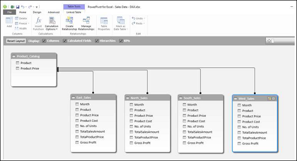
สมมติว่าคุณมีข้อมูลการขายของผลิตภัณฑ์ตามภูมิภาคในตารางข้อมูลและยังมีแคตตาล็อกผลิตภัณฑ์ในแบบจำลองข้อมูล
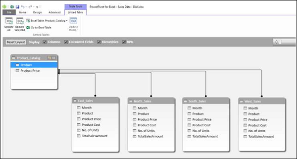
สร้าง Power PivotTable ด้วยข้อมูลนี้

ดังที่คุณสังเกตได้ Power PivotTable ได้สรุปข้อมูลการขายจากทุกภูมิภาค สมมติว่าคุณต้องการทราบผลกำไรขั้นต้นของผลิตภัณฑ์แต่ละรายการ คุณทราบราคาของผลิตภัณฑ์แต่ละรายการต้นทุนที่ขายและจำนวนหน่วยที่ขาย

อย่างไรก็ตามหากคุณต้องการคำนวณกำไรขั้นต้นคุณต้องมีคอลัมน์อีกสองคอลัมน์ในแต่ละตารางข้อมูลของภูมิภาค - ราคาผลิตภัณฑ์รวมและกำไรขั้นต้น เนื่องจาก PivotTable ต้องการคอลัมน์ในตารางข้อมูลเพื่อสรุปผลลัพธ์
ดังที่คุณทราบราคาผลิตภัณฑ์ทั้งหมดคือราคาผลิตภัณฑ์ * จำนวนหน่วยและกำไรขั้นต้นคือจำนวนเงินทั้งหมด - ราคาผลิตภัณฑ์ทั้งหมด
คุณต้องใช้นิพจน์ DAX เพื่อเพิ่มคอลัมน์จากการคำนวณดังนี้ -
คลิกแท็บ East_Sales ในมุมมองข้อมูลของหน้าต่าง Power Pivot เพื่อดูตารางข้อมูล East_Sales
คลิกแท็บออกแบบบน Ribbon
คลิกเพิ่ม
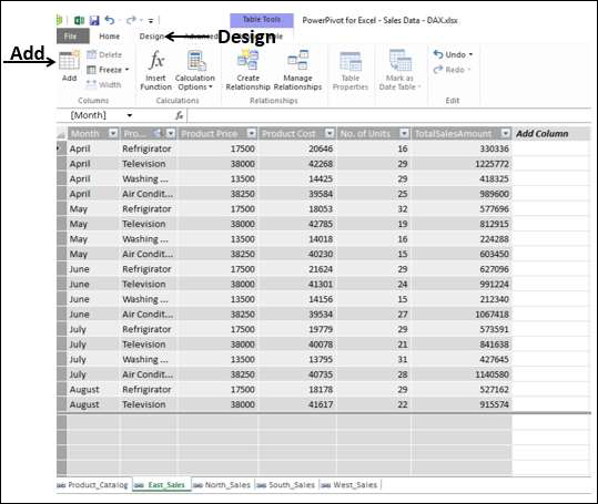
คอลัมน์ทางด้านขวาพร้อมส่วนหัว - เพิ่มคอลัมน์จะถูกเน้น
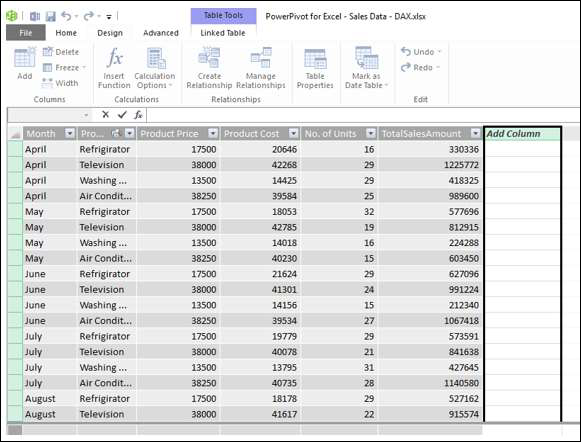
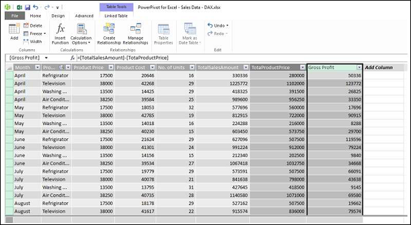
ประเภท = [Product Price] * [No. of Units] ในแถบสูตรแล้วกด Enter.

คอลัมน์ใหม่ที่มีส่วนหัว CalculatedColumn1 แทรกด้วยค่าที่คำนวณโดยสูตรที่คุณป้อน

ดับเบิลคลิกที่ส่วนหัวของคอลัมน์จากการคำนวณใหม่
เปลี่ยนชื่อส่วนหัวเป็น TotalProductPrice.
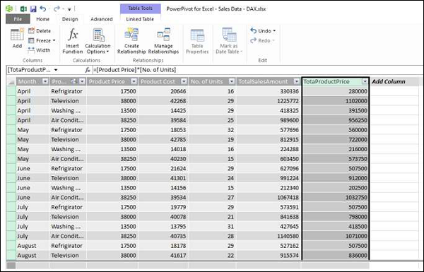
เพิ่มคอลัมน์จากการคำนวณอีกหนึ่งคอลัมน์สำหรับกำไรขั้นต้นดังนี้ -
คลิกแท็บออกแบบบน Ribbon
คลิกเพิ่ม
คอลัมน์ทางด้านขวาพร้อมส่วนหัว - เพิ่มคอลัมน์จะถูกเน้น
ประเภท = [TotalSalesAmount] − [TotaProductPrice] ในแถบสูตร
กดปุ่มตกลง.
คอลัมน์ใหม่ที่มีส่วนหัว CalculatedColumn1 แทรกด้วยค่าที่คำนวณโดยสูตรที่คุณป้อน

ดับเบิลคลิกที่ส่วนหัวของคอลัมน์จากการคำนวณใหม่
เปลี่ยนชื่อส่วนหัวเป็นกำไรขั้นต้น
เพิ่มคอลัมน์จากการคำนวณในไฟล์ North_Salesตารางข้อมูลในลักษณะเดียวกัน การรวมขั้นตอนทั้งหมดดำเนินการดังนี้ -
คลิกแท็บออกแบบบน Ribbon
คลิกเพิ่ม คอลัมน์ทางด้านขวาพร้อมส่วนหัว - เพิ่มคอลัมน์จะถูกเน้น
ประเภท = [Product Price] * [No. of Units] ในแถบสูตรแล้วกด Enter
คอลัมน์ใหม่ที่มีส่วนหัว CalculatedColumn1 ถูกแทรกด้วยค่าที่คำนวณโดยสูตรที่คุณป้อน
ดับเบิลคลิกที่ส่วนหัวของคอลัมน์จากการคำนวณใหม่
เปลี่ยนชื่อส่วนหัวเป็น TotalProductPrice.
คลิกแท็บออกแบบบน Ribbon
คลิกเพิ่ม คอลัมน์ทางด้านขวาพร้อมส่วนหัว - เพิ่มคอลัมน์จะถูกเน้น
ประเภท = [TotalSalesAmount] − [TotaProductPrice]ในแถบสูตรแล้วกด Enter คอลัมน์ใหม่ที่มีส่วนหัวCalculatedColumn1 แทรกด้วยค่าที่คำนวณโดยสูตรที่คุณป้อน
ดับเบิลคลิกที่ส่วนหัวของคอลัมน์จากการคำนวณใหม่
เปลี่ยนชื่อส่วนหัวเป็น Gross Profit.
ทำซ้ำขั้นตอนที่ระบุข้างต้นสำหรับตารางข้อมูล South Sales และตารางข้อมูล West Sales
คุณมีคอลัมน์ที่จำเป็นในการสรุปกำไรขั้นต้น ตอนนี้สร้าง Power PivotTable

คุณสามารถสรุปไฟล์ Gross Profit ซึ่งกลายเป็นไปได้ด้วยคอลัมน์จากการคำนวณใน Power Pivot และทั้งหมดนี้สามารถทำได้ในไม่กี่ขั้นตอนที่ปราศจากข้อผิดพลาด
You can summarize it region wise for the products as given below also −

Calculated Field
Suppose you want to calculate the percentage of profit made by each region product-wise. You can do so by adding a calculated field to the Data Table.
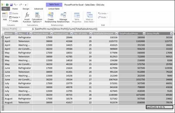
Click below the column Gross Profit in the East_Sales table in Power Pivot window.
Type EastProfit: = SUM ([Gross Profit]) / sum ([TotalSalesAmount]) in the formula bar.
Press Enter.

The calculated field EastProfit is inserted below the Gross Profit column.
Right click the calculated field − EastProfit.
Select Format from the dropdown list.

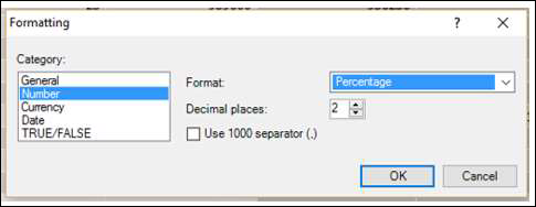
The Formatting dialog box appears.
Select Number under Category.
In the Format box, select Percentage and click OK.
The calculated field EastProfit is formatted to percentage.
Repeat the steps to insert the following calculated fields −
NorthProfit in North_Sales data table.
SouthProfit in South_Sales data table.
WestProfit in West_Sales data table.
Note − You cannot define more than one calculated field with a given name.
Click on the Power PivotTable. You can see that the calculated fields appear in the tables.

Select the fields − EastProfit, NorthProfit, SouthProfit and WestProfit from the tables in the PivotTable Fields list.
Arrange the fields such that the Gross Profit and Percentage Profit appear together. The Power PivotTable looks as follows −

Note − The Calculate Fields were called Measures in earlier versions of Excel.