3D-Transformation

Drehung

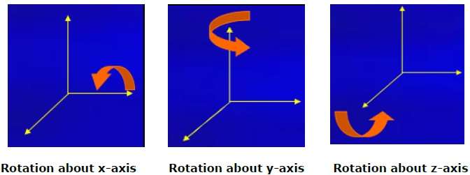
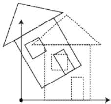
3D-Rotation ist nicht dasselbe wie 2D-Rotation. Bei der 3D-Drehung müssen wir den Drehwinkel zusammen mit der Drehachse angeben. Wir können eine 3D-Drehung um die X-, Y- und Z-Achse durchführen. Sie werden in der Matrixform wie folgt dargestellt -

$$ R_ {x} (\ theta) = \ begin {bmatrix} 1 & 0 & 0 & 0 \\ 0 & cos \ theta & −sin \ theta & 0 \\ 0 & sin \ theta & cos \ theta & 0 \\ 0 & 0 & 0 & 1 \ \ \ end {bmatrix} R_ {y} (\ theta) = \ begin {bmatrix} cos \ theta & 0 & sin \ theta & 0 \\ 0 & 1 & 0 & 0 \\ −sin \ theta & 0 & cos \ theta & 0 \\ 0 & 0 & 0 & 1 \\ \ end {bmatrix} R_ {z} (\ theta) = \ begin {bmatrix} cos \ theta & −sin \ theta & 0 & 0 \\ sin \ theta & cos \ theta & 0 & 0 \\ 0 & 0 & 1 & 0 \\ 0 & 0 & 0 & 1 \ end {bmatrix} $$

Die folgende Abbildung erklärt die Drehung um verschiedene Achsen -

Skalierung

Sie können die Größe eines Objekts mithilfe der Skalierungstransformation ändern. Während des Skalierungsprozesses erweitern oder komprimieren Sie die Abmessungen des Objekts. Die Skalierung kann erreicht werden, indem die ursprünglichen Koordinaten des Objekts mit dem Skalierungsfaktor multipliziert werden, um das gewünschte Ergebnis zu erhalten. Die folgende Abbildung zeigt den Effekt der 3D-Skalierung -

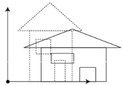
Bei der 3D-Skalierung werden drei Koordinaten verwendet. Nehmen wir an, dass die ursprünglichen Koordinaten (X, Y, Z) sind, die Skalierungsfaktoren $ (S_ {X,} S_ {Y,} S_ {z}) $ sind und die erzeugten Koordinaten (X ', Y' sind. , Z '). Dies kann mathematisch wie unten dargestellt dargestellt werden -

$ S = \ begin {bmatrix} S_ {x} & 0 & 0 & 0 \\ 0 & S_ {y} & 0 & 0 \\ 0 & 0 & S_ {z} & 0 \\ 0 & 0 & 0 & 1 \ end {bmatrix} $

P '= P ∙ S.

$ [{X} '\: \: \: {Y}' \: \: \: {Z} '\: \: \: 1] = [X \: \: \: Y \: \: \: Z \: \: \: 1] \: \: \ begin {bmatrix} S_ {x} & 0 & 0 & 0 \\ 0 & S_ {y} & 0 & 0 \\ 0 & 0 & S_ {z} & 0 \\ 0 & 0 & 0 & 1 \ end {bmatrix} $

$ = [X.S_ {x} \: \: \: Y.S_ {y} \: \: \: Z.S_ {z} \: \: \: 1] $

Scheren

Eine Transformation, die die Form eines Objekts neigt, wird als bezeichnet shear transformation. Wie bei der 2D-Scherung können wir ein Objekt entlang der X-Achse, Y-Achse oder Z-Achse in 3D scheren.

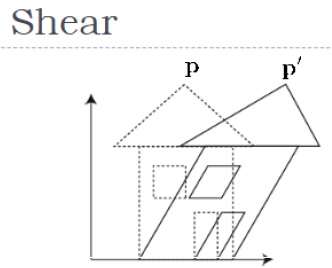
Wie in der obigen Abbildung gezeigt, gibt es eine Koordinate P. Sie können sie scheren, um eine neue Koordinate P 'zu erhalten, die in 3D-Matrixform wie folgt dargestellt werden kann:

$ Sh = \ begin {bmatrix} 1 & sh_ {x} ^ {y} & sh_ {x} ^ {z} & 0 \\ sh_ {y} ^ {x} & 1 & sh_ {y} ^ {z} & 0 \\ sh_ {z} ^ {x} & sh_ {z} ^ {y} & 1 & 0 \\ 0 & 0 & 0 & 1 \ end {bmatrix} $

P '= P ∙ Sh

$ X '= X + Sh_ {x} ^ {y} Y + Sh_ {x} ^ {z} Z $

$ Y '= Sh_ {y} ^ {x} X + Y + sh_ {y} ^ {z} Z $

$ Z '= Sh_ {z} ^ {x} X + Sh_ {z} ^ {y} Y + Z $

Transformationsmatrizen

Die Transformationsmatrix ist ein grundlegendes Werkzeug für die Transformation. Eine Matrix mit nxm Dimensionen wird mit der Koordinate von Objekten multipliziert. Normalerweise werden 3 x 3 oder 4 x 4 Matrizen zur Transformation verwendet. Betrachten Sie beispielsweise die folgende Matrix für verschiedene Operationen.

$ T = \ begin {bmatrix} 1 & 0 & 0 & 0 \\ 0 & 1 & 0 & 0 \\ 0 & 0 & 1 & 0 \\ t_ {x} & t_ {y} & t_ {z} & 1 \\ \ end {bmatrix} $	$ S = \ begin {bmatrix} S_ {x} & 0 & 0 & 0 \\ 0 & S_ {y} & 0 & 0 \\ 0 & 0 & S_ {z} & 0 \\ 0 & 0 & 0 & 1 \ end {bmatrix} $	$ Sh = \ begin {bmatrix} 1 & sh_ {x} ^ {y} & sh_ {x} ^ {z} & 0 \\ sh_ {y} ^ {x} & 1 & sh_ {y} ^ {z} & 0 \\ sh_ {z} ^ {x} & sh_ {z} ^ {y} & 1 & 0 \\ 0 & 0 & 0 & 1 \ end {bmatrix} $
Translation Matrix	Scaling Matrix	Shear Matrix
$ R_ {x} (\ theta) = \ begin {bmatrix} 1 & 0 & 0 & 0 \\ 0 & cos \ theta & -sin \ theta & 0 \\ 0 & sin \ theta & cos \ theta & 0 \\ 0 & 0 & 0 & 1 \\ \ end {bmatrix} $	$ R_ {y} (\ theta) = \ begin {bmatrix} cos \ theta & 0 & sin \ theta & 0 \\ 0 & 1 & 0 & 0 \\ -sin \ theta & 0 & cos \ theta & 0 \\ 0 & 0 & 0 & 1 \\ \ end {bmatrix} $	$ R_ {z} (\ theta) = \ begin {bmatrix} cos \ theta & -sin \ theta & 0 & 0 \\ sin \ theta & cos \ theta & 0 & 0 \\ 0 & 0 & 1 & 0 \\ 0 & 0 & 0 & 1 \ end {bmatrix} $
Rotation Matrix